Getting started guide
Getting started guideIntroductionInstallation et lancement de Talren v6Architecture of the interfaceProjectGeometrySoil characteristicsLoadsReinforcementsStaged construction (Phases and Situations)PhasesSituationsCalculation methodSet of safety factorsRange of surfaces to be examinedSeismic conditionsCase study: Stability of a temporary slopeTheoretical reminder: How to manage the security level in traditional method?Case study descriptionHow to start with Talren v6Defining a new projectProject definitionDefinition of geometryDefinition of soil propertiesDefinition of loadsTraditional methodStage 1: without water table or loadStage 2: Influence of a external load on the surfaceStage 3: Influence of a horizontal water tableStage 4: Influence of a water table drawdownStage 5: Interest of a water table control systemStage 1 / Situation 2: calcul à la rupture (méthode cinématique)Eurocode approachHow to use a set of partial coefficients?Stage 6 (identical to Phase 1): Without water table or loadingSituation 1: traditional methodSituation 2: Yield design calculation (kinematic method) with imposed XFSituation 3: Yield design calculation (kinematic method) with automatic XF searchWant to go further?
Introduction
The aim of this document is to give a quick overview of the Talren v6 interface by giving a quick but detailed overview of the interface to clarify the principle of its use while describing the main features.
The practical case of the stability of a temporary slope will be handled: firstly on the basis of the traditional method and secondly by introducing the safety required by the Eurocode, while comparing Bishop's method (slice method) and the kinematic method of yield design.
Installation et lancement de Talren v6
First of all, it is necessary to install Talren v6 on the user workstation.
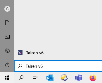
To know if Talren v6 is installed on your computer, click on the Start Menu and simply write Talren v6:
If Talren is not installed on your computer, please download it from our website (see Downloads on the right menu): https://www.terrasol.fr/catalogue/talren-v6
Once Talren v6 is installed on the computer, it can be launched in:
Demostration mode: the interface can be used with limited functionality (the calculation cannot be started, the project cannot be saved or printed).
Trial mode: this mode allows the use of all features, including the launch of the calculation, but does not allow the saving of projects or the printing of the report.
To request an evaluation license, please apply via this form: https://www.terrasol.fr/logiciels/talren-evaluation-request
Once the form is completed and validated, you will receive by email the instructions to follow.
The evaluation license will be usable for 30 days from the first use.
Professional license mode: this mode requires a professional license that allows you to use all the features of Talren v6.
If you wish to receive a technical-commercial proposal (quotation) to acquire a professional license, you can make a request via this form: https://www.terrasol.fr/logiciels/devis
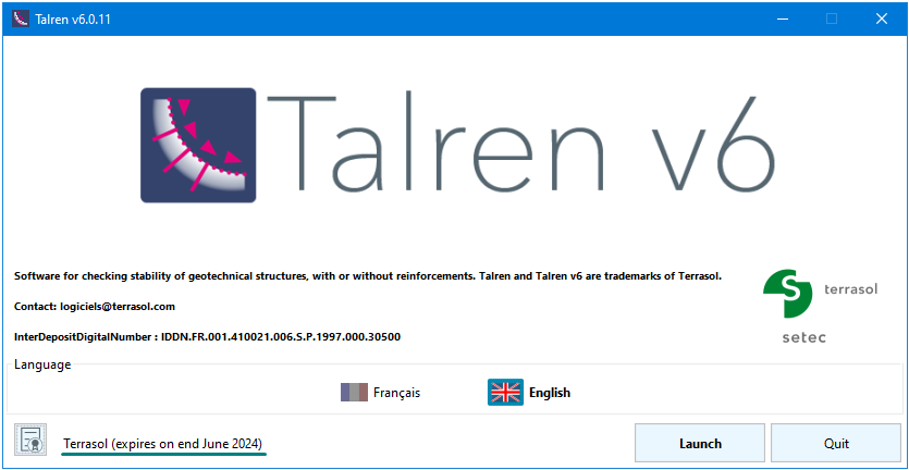
At launch, you will be able to read the name of your company and, if it exists, the expiration date of your key.
Architecture of the interface
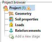
The interface dashboard is composed of the following sections:
- Project tree and properties (red and green areas)
- Drawing area (blue area)
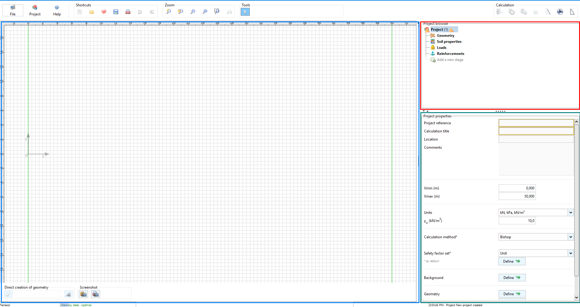
At the top right of the interface dashboard, the interface presents the navigation menu that allows access to all the categories that define the project in particular:
- General project properties
- Geometry
- Soil characteristics
- Surcharges
- Reinforcements
- Phases / Situations
Project
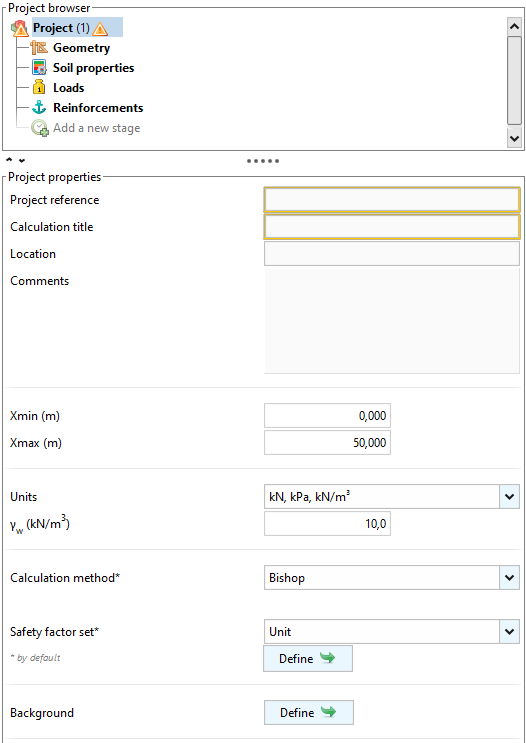
This category allows you to define general properties of the project, in particular:
- Project number
- Title of the calculation
- Location
- Comment
These properties are optional and will be included in the print report.
The left and right boundaries of the geometric model are defined by its boundary abscissa:
The following properties are default values for the current project (they will be proposed by default when creating new phases/situations):
System of units, several choices available:
- kN, kPa, kN/m³
- MN, MPa, MN/m³
- t, t/m², t/m³
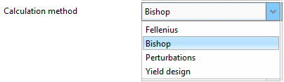
Calculation method, several choices available:
- Bishop (slice method)
- Fellenius (slice method)
- Perturbations (global method)
- Yield design (kinematic method)
Set of safety coefficients: about twenty possible choices, it is however possible to define a personalized set of coefficients
Talren also allows the import of a background (image .jpeg or .png) on which the user can define the geometry with the mouse.
Geometry
This category allows the entry of points and segments that define the geometry of the project.
Several options are available:
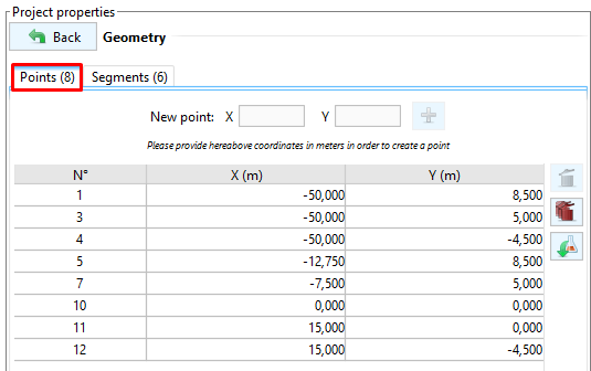
Input via table filling:
- The points are defined by their X and Y coordinates, which are entered in the Points tab
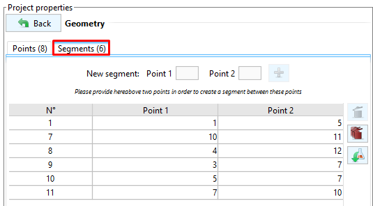
- The points are connected by segments to be defined in the Segments tab
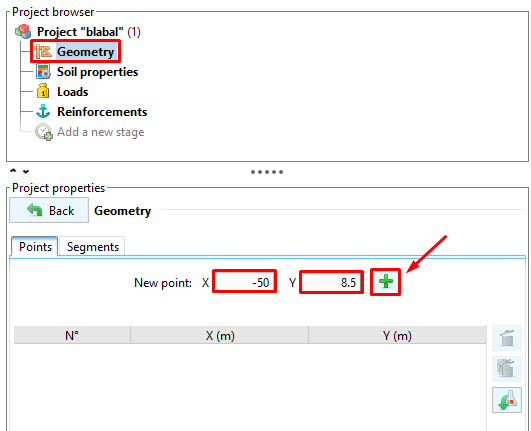
Input on the lower part of the drawing area via the edit bar:
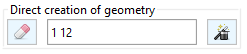
It is necessary to enter here the coordinates X [m] and Y [m] of the new points to create (for example here: X=1m and Y=12m)
Input via the mouse directly on the drawing area using the button bar:
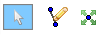
- The first button is used to move around the drawing area
- The second button allows to define new points and to draw new segments
- The third button allows to move already defined points
Soil characteristics
This category allows you to define soil layers as materials based on the following parameters:
| Parameter | Unit | Description |
|---|---|---|
| kN/m³ | Density of the soil | |
| kPa | Soil cohesion | |
| kPa/m | Cohesion increment with depth | |
| ° | Friction angle |
The cohesion is to be characterized as effective or undrained, this has an influence on the level of safety to be considered (the value will be fixed by the set of safety coefficients chosen later on in the Situation).
It is possible to define an anisotropy of the cohesion: this allows to adjust its value according to the inclination of the tangent to the fracture surface with respect to the horizontal.
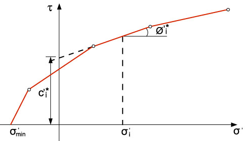
The friction angle can be defined by a constant value (choice "Linear") or adjusted by a customized breaking criterion defined by a set of couples (σ,τ).
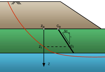
If nails are present, additional parameters must be defined:
| Parameter | Unit | Description |
|---|---|---|
| kPa | Axial friction limit that can be mobilized along the nails (wizard available) | |
| kPa | Maximum pressure that can be developed by the soil under transversal loading | |
| kPa | Frontal reaction coefficient ( wizard available) |
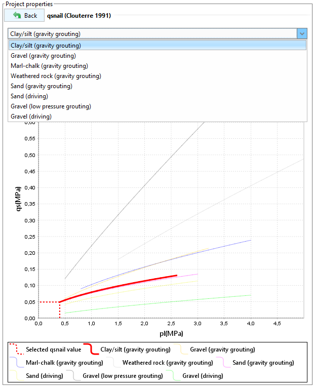
A wizard for defining qs is available to allow the use of correlations between the limit pressure pl [MPa] and qs [MPa] proposed by the Clouterre 1991 recommendations:
It is possible to define specific safety coefficients for each soil layer, in particular on the self-weight, on the cohesion and on tan(φ). These coefficients take precedence over those of the set of safety coefficients used for each situation.
In the case of a flow calculation, it is also possible to allow the flow within the soil layer by defining its horizontal kh [m/s] and vertical kv [m/s] permeabilities.
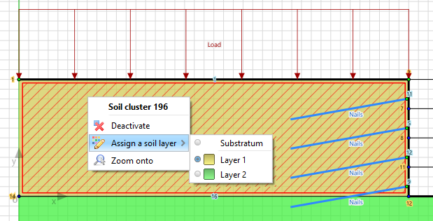
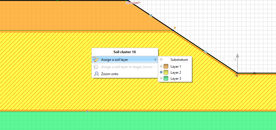
The soil layer can be associated with a volume in the drawing area in two different ways:
- With a "drag and drop" of the "Layer" label
- By right-clicking on the volume in the drawing area and making a choice in Assign soil layer
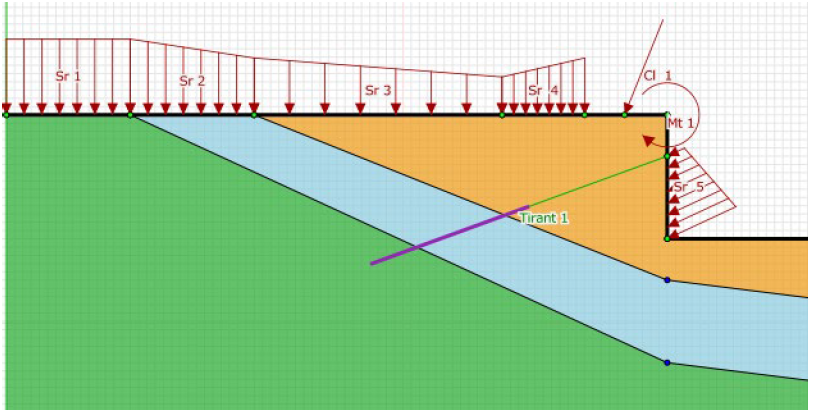
Loads
This section allows to define the external loads to be considered in the stability calculation:
- Distributed overloads: these are localized distributed overloads defined between two points of the model and characterized by a load variation between these two points.
- Linear loads: these are the forces (Q) applied at a given point (X, Y), possibly inclined by an angle (º) to the horizontal. In the case of the use of slice methods, it is necessary to characterize its diffusion in the soil (this is not used in the kinematic method of calculation at failure).
- Linear moments: these are the moments (M) applied to a given point (X, Y).
It is possible to define families of overloads: this allows to manipulate the set of overloads in order to take advantage of common properties, with the possibility to create exceptions on particular elements.
Reinforcements
Four types of reinforcement can be identified within this category:
- Nails: these are elements that can work in tension/compression and shear
- Anchors: these are reinforcement elements that can only work in traction
- Strips: these are reinforcement elements that can only work in traction
- Buttons: these are external elements that can only work in compression
All reinforcements, except for struts, interact with the surrounding soil. It is therefore necessary to enter the necessary parameters to define this reinforcement/soil interaction.
It is possible to define families of reinforcements: this allows to manipulate the set of reinforcements in order to take advantage of common properties, with the possibility to create exceptions on particular elements.
Staged construction (Phases and Situations)
The stability analysis is divided into phases and situations:
- A phase is a stage of the project.
- A situation is a way to analyze the stability of the structure at a given phase.
Practical rule for deciding whether to define a new phase or a new situation is sufficient: as soon as the configuration/layout under consideration requires changing the graphical representation on the drawing space, a new phase should be defined.
Phases
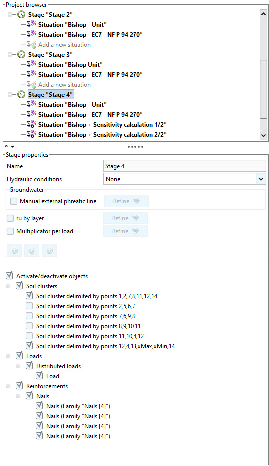
As previously mentioned, a phase corresponds to a stage of the project.
It is possible to activate or deactivate elements of the model such as reinforcements, loads or soil volumes by associating them with a previously defined soil layer.
The same geometric volume can contain different soil layers over several phases.
This activation/deactivation can be done directly by clicking on the drawing area or via the phase tree:
The hydraulic conditions are to be defined within the phase, several options are available:
- None: no hydraulic conditions will be considered
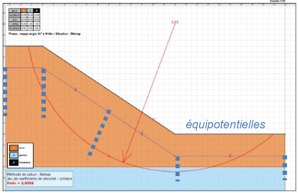
- Water table: the pore pressures will be calculated at any point in a hydrostatic way with respect to the water table defined from a polyline (points X, Y) with the possibility of defining the orientation of the equipotentials (angle in degrees with respect to the horizontal)
- Pressures given along a polygonal rupture surface: only valid for situations that aim to examine a very specific rupture mechanism defined by a concatenation of segments connecting points (X, Y) entered by the user
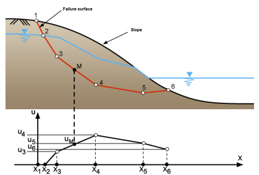
- Imported or manual triangular pore pressure mesh: this mode allows you to manually define or import a pore pressure mesh from a text/paper-press file or even from Plaxis. The mesh will be perfectly defined by nodes, triangles systematically linking 3 nodes and the pore pressure values at each node.
Calculated pore pressure triangular mesh (new): this mode allows an integrated calculation, in steady state, of the pore pressure field to be considered for stability analyses. The calculation is based on a numerical resolution of the Laplace equation taking into account the multilayer and anisotropic character of the ground. Here is an example of flow networks within a dam and around a retaining wall:
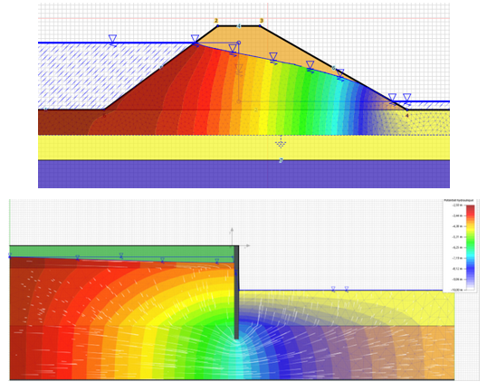
It is also possible to define a bottom of the water table below which the pore pressures will be considered null. This is useful in case of a tight bottom inside which the flow cannot occur.
Situations
As mentioned before, a situation is a way to analyze the stability of the structure at a given phase.
Calculation method
For this, you have to choose a calculation method, several choices are possible:
Bishop or Fellenius (slice methods): the soil is broken down into vertical slices and the force and moment equilibrium of each slice and the global moment equilibrium are solved. These two methods differ in the assumption on the inclination of the inter-slice reaction:
- Bishop assumes zero slope of the inter-slice reaction
- Fellenius assumes a slope of the inter-slice reaction parallel to the base of the slice
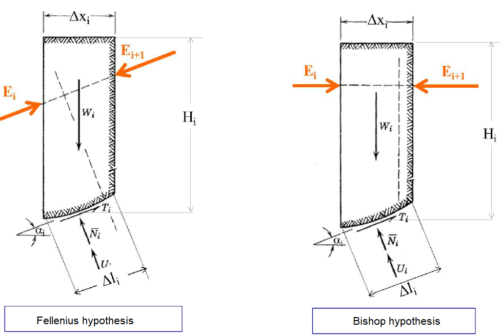
These methods require additional hypotheses whose favourable or unfavourable character with respect to stability cannot be controlled, in particular the inclination of the inter-trench reaction and the diffusion of the loads and forces mobilized in the reinforcements.
Perturbations (global method): this method was developed by Raulin, Rouques, Toubol (1974). It is a calculation method for non-circular failure of any shape. The complementary hypothesis that characterizes it concerns the value of the effective normal stress. This is expressed as a function of the effective normal stress deduced from the Fellenius method.
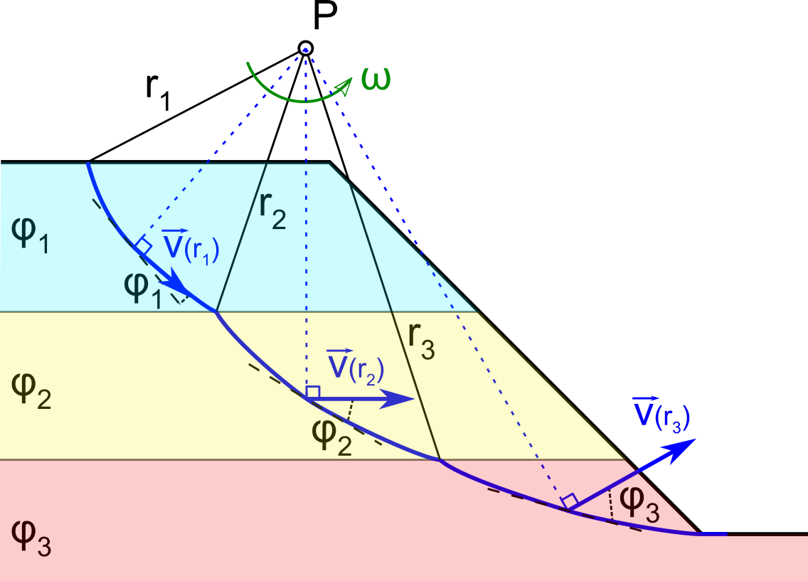
Yield design (kinematic method): this calculation method represents a kinematic approach from the outside of the failure load of geotechnical structures. This approach is developed within the framework of the general theory of calculation at failure which was formalized by J. Salençon (1983).
Set of safety factors
The calculation of the situation requires the consideration of a set of safety coefficients on the quantities involved in the calculation. The choice is to be made from the set of coefficients that have been "activated" or chosen in the Project category.
In the definition of the situation, it is possible to view the values of the safety coefficients without being able to modify them (they can be modified in the Project category):
Range of surfaces to be examined
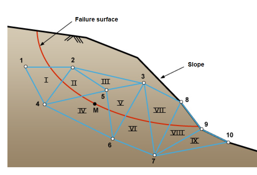
The stability calculation proposed by Talren is performed on a set of surfaces prefixed by the user in the form of a range. Talren allows the easy generation of these ranges:
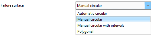
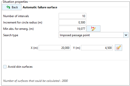
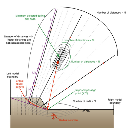
Automatic circular: this is a quick way to examine the stability for a predefined set of surfaces automatically generated by the interface for the following parameters:
Number of intervals (N): number of directions examined and number of centers examined in each direction
Increment on radius: distance to be added (positive value) or subtracted (if negative value) on the initial radius determined by the distance between the examined center and the first point to be impacted on the field
Bounding emergence abscissa: the value of the abscissa X to the right of which the surfaces to be retained must end. In other words, all surfaces terminating to the left of this value of X will be discarded.
Search type, two possible choices to determine the first point to target for the first surface generated apart from each potential center
- Imposed passage point (X, Y)
- Circles tangent to a layer (layer to choose among those defined in the model)
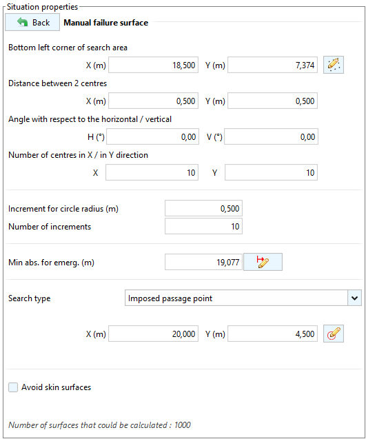
- Manual circular: define a set of circular surfaces generated from a grid of potential centers by examining several possible radii
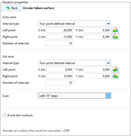
Manual circular with intervals: here you define the set of start (entry interval) and end (exit interval) points of the surface. Talren will deduce the center and radius for each pair of entry and exit points and the angle at which these two points are "seen" (exploration) in order to generate the range to be examined.
Each interval can be reduced to a single point, in which case an interval type of Punctual should be chosen.
- Polygonal: this is a surface described by a series of points (X, Y). This type of surface can be used to examine very specific mechanisms or those that are observed in situ.
- Logarithmic spirals: these mechanisms are proposed only in the case of the kinematic method of calculation at break. Each logarithmic spiral is defined from an entry point (belonging to the entry interval), an exit point (belonging to an exit interval) and an angle at the pole. Talren is able to examine surfaces with upward or downward concavity.
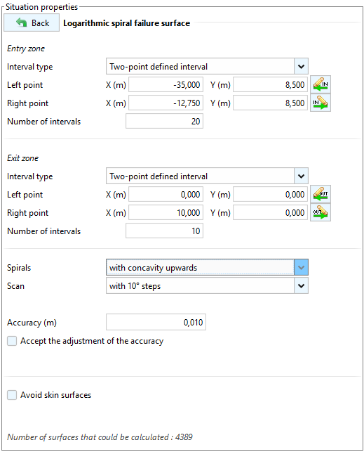
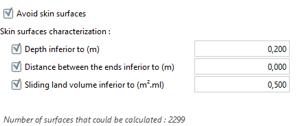
All of the previous options offer the possibility of discarding skin surfaces based on additional criteria:
Seismic conditions
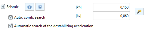
It is also possible to integrate inertial effects under seismic conditions. For this, it is necessary to define the seismic acceleration ratios:
| Parameter | Unit | Description |
|---|---|---|
| - | Horizontal seismic coefficient ( | |
| - | Vertical seismic coefficient ( |
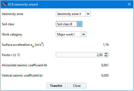
Talren v6 proposes an earthquake assistant in accordance with Eurocode 8 which allows to estimate these seismic coefficients according to the seismicity zone (1 to 5), the soil class (A to E), the category of the structure (I to IV) and the "r" factor:
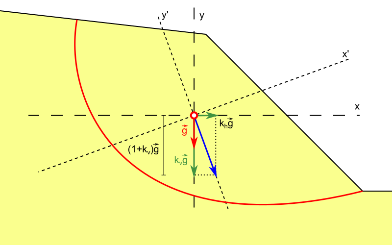
The following help figures are integrated in the interface to represent the effect of these seismic coefficients and where they are applied (soil and water):
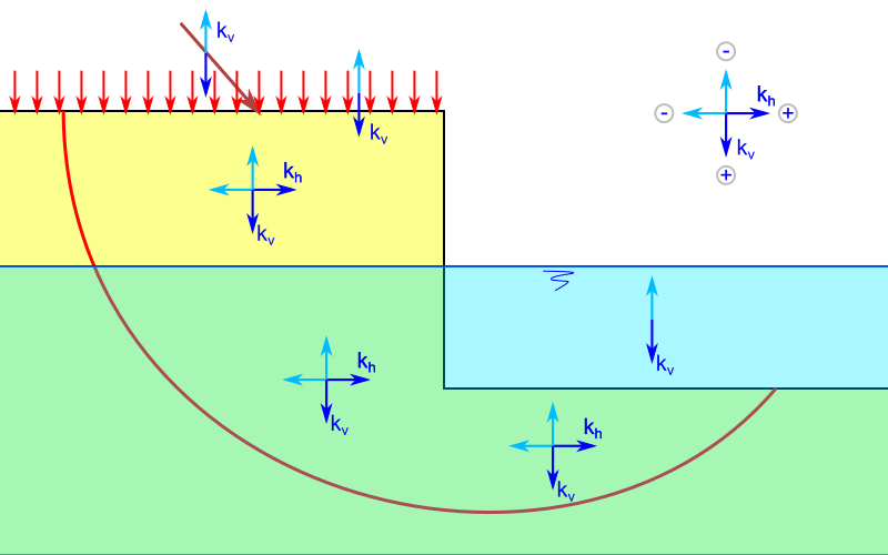
Talren v6 allows to examine all possible kH and kV combinations.
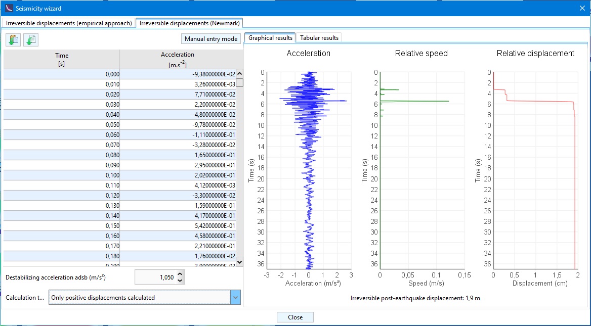
It also allows to automatically search for the destabilizing acceleration: the one that leads to the limit equilibrium and that can feed an irreversible displacement calculation.
The earthquake assisant  available at the top right of the interface offers an estimation of the irreversible displacement by different methods:
Empirical approaches:
- Ambraseys et Menu (1988)
- Jibson (2007)
- Lazari et Padopoulos (2012)
Newmark's method:
Case study: Stability of a temporary slope
This practical use case of the interface serves several purposes:
- Define and manipulate a simple project with Talren v6
- How to manage the safety level in traditional method?
- Analyze the evolution of the safety factor throughout the proposed calculation phase
- Propose a solution with a sheet control system
- Stability analysis using a set of partial coefficients according to Eurocode 7
- Comparison with the kinematic method of calculation at failure
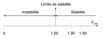
Theoretical reminder: How to manage the security level in traditional method?
In the traditional approach (partial coefficients equal to 1.00), the security level usually sought is:
How should we physically interpret the result obtained with Talren?
In general, the higher the security, the lower the deformations.
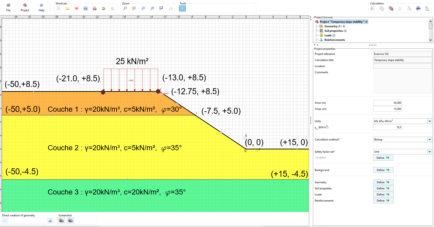
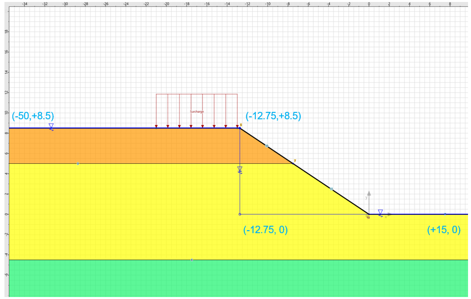
Case study description
We wish to study the stability of this temporary embankment under different loading conditions using the traditional method:
- Phase 1: Without water table or loading
- Phase 2: Influence of a external load on the surface
- Phase 3: Influence of a horizontal water table
- Phase 4: Influence of a water table drawdown
- Phase 5: Interest of a water table control system
- Phase 1 / Situation 2: Use of the kinematic method of yield design
We wonder what is the evolution of the stability coefficient with respect to the overall stability.
Then, we will be interested in examining the stability with a Eurocode approach using an additional phase:
- Phase 6: Use of a set of partial coefficient
How to start with Talren v6
Defining a new project
Launch Talren v6 and click on the New project... button in the dashboard or in the File menu.
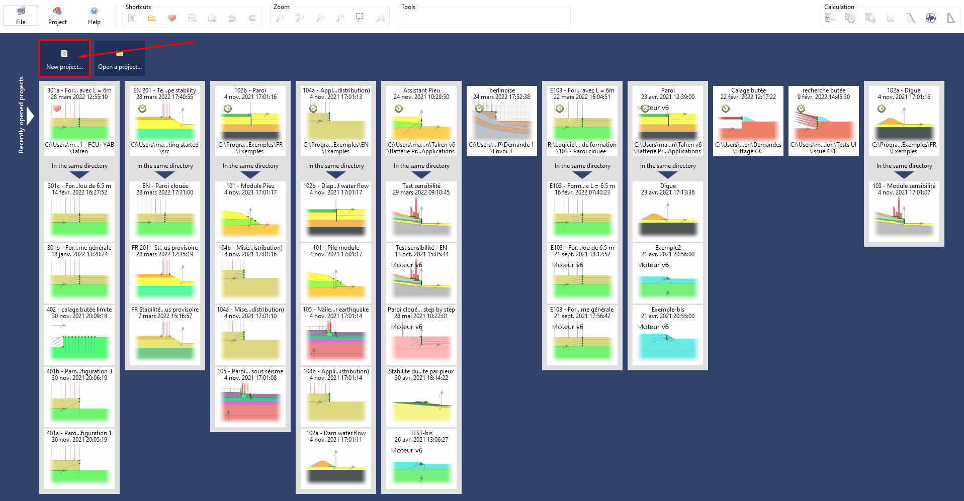
The interface dashboard is composed of 3 sections:
- Drawing area (blue zone)
- Project tree (red area)
- Project category properties pane (green area)
Project definition
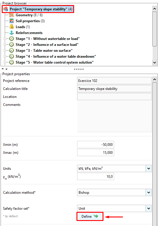
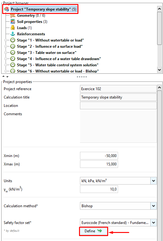
We start by defining the project properties.
To do this, click on the Project category of the tree (red zone) and input the following data:
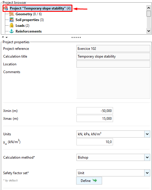
In the traditional method, we will use a unit weighting.
For safety factor sets, it is advisable to check Unitary:
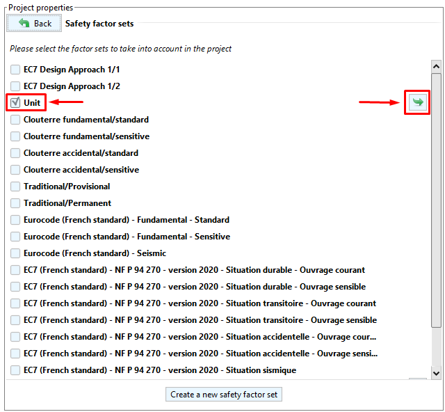
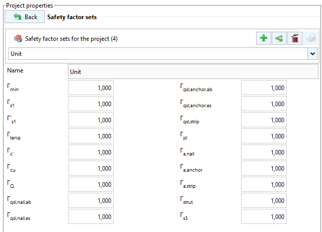
By clicking on the arrow on the right, you can view the safety coefficients (units):
Definition of geometry
In the Geometry category, please enter the coordinates of the points in the Points tab and click on the  :
:
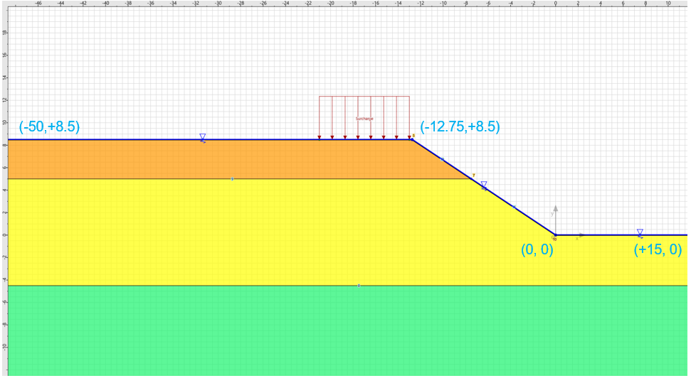
Below are all the coordinates of the points to be entered:
Here are the completed point and segment tables:
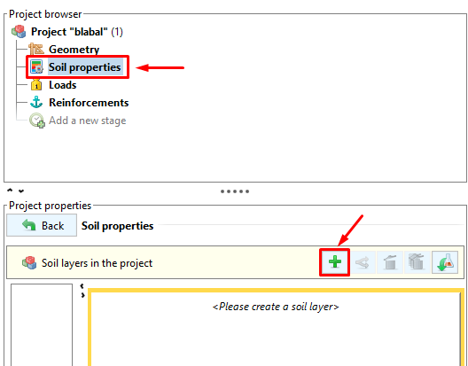
Definition of soil properties
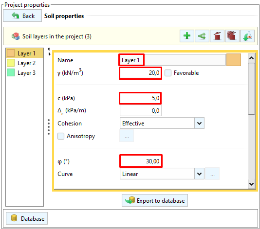
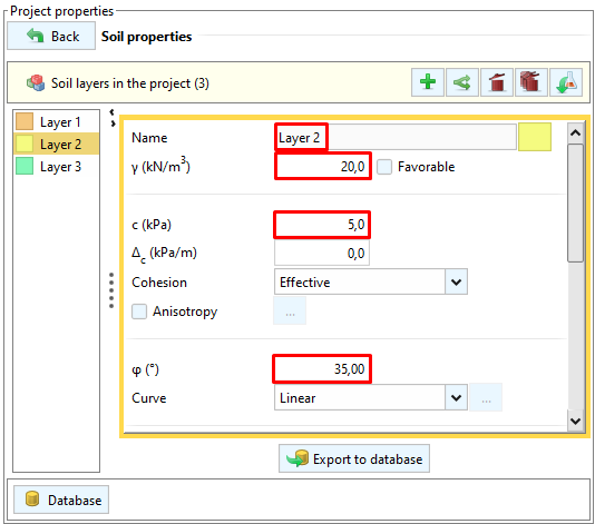
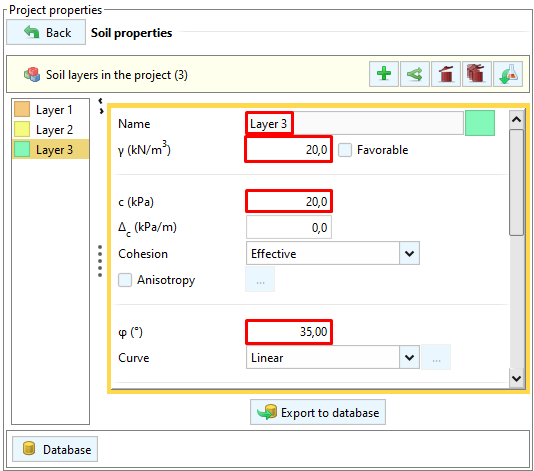
We will then define the characteristics of the soils:
| kN/m³ | kN/m² | º | |
| Soil layer 1 | 20 | 5 | 30 |
| Soil layer 2 | 20 | 5 | 35 |
| Soil layer 3 | 20 | 20 | 35 |
To create a new layer, click on the button :
Then enter the characteristics of each layer:
To assign the soil layers to the soil volumes defined in the Geometry category, we can drag and drop the layers onto the volumes or right click on the volumes and assign them the desired soil layer:
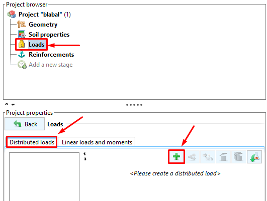
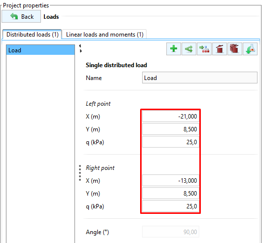
Definition of loads
We will then define a 25 kPa surcharge on the surface over a length of 8 m.
To do this, we will add a new distributed surcharge using the button :
Here are the values to enter:
Traditional method
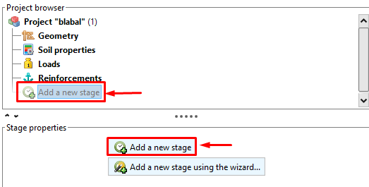
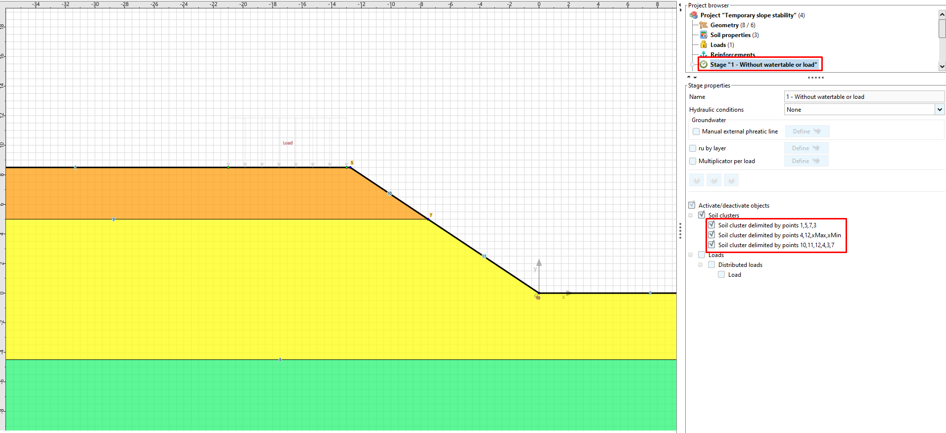
Stage 1: without water table or load
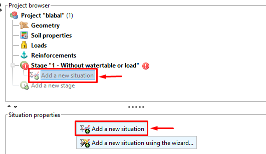
We are going to define a first calculation phase by clicking on Add a new phase in the project tree and then in the bottom button Add a new phase:
Stage properties:
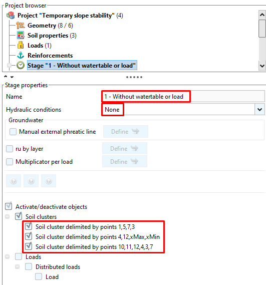
We will activate only the 3 soil volumes. This can be done by activating each element in the list at the bottom or by left-clicking on the drawing.
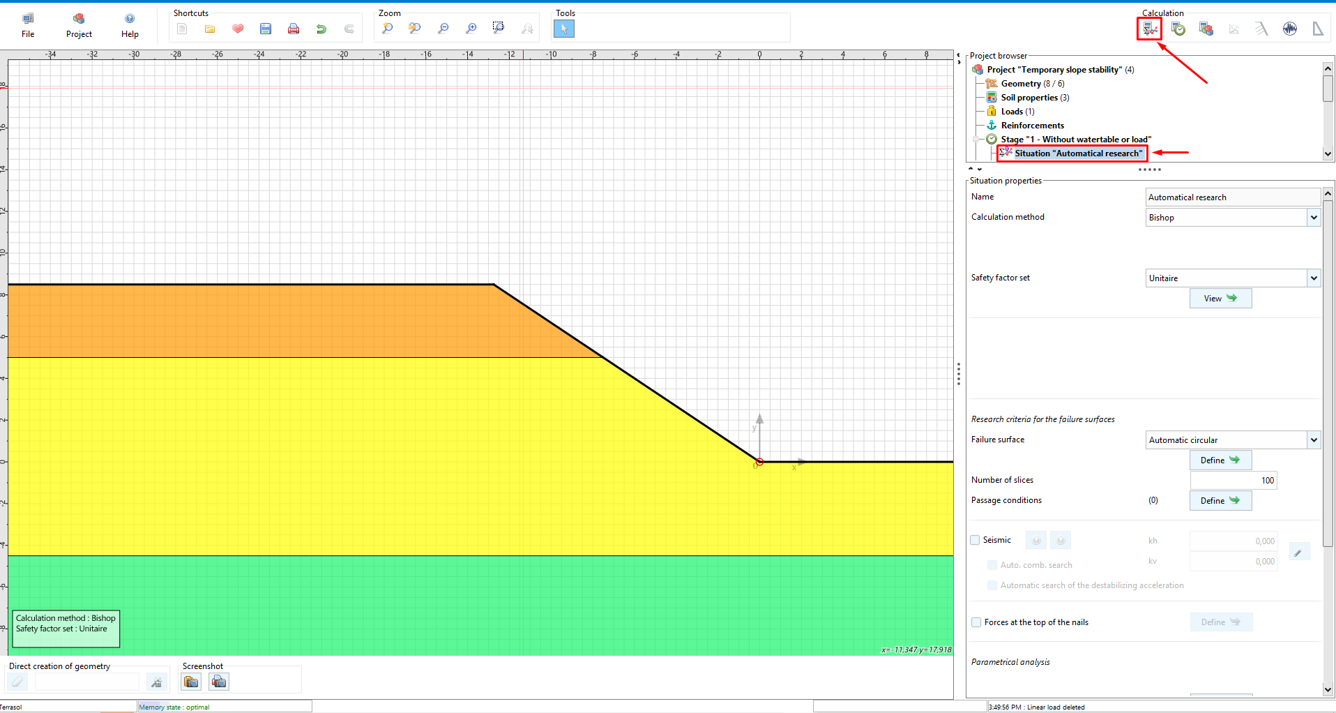
We will define a new situation within this first phase:
We will do a first situation using Bishop's method, using a unit weighting and using an automatic circular search:
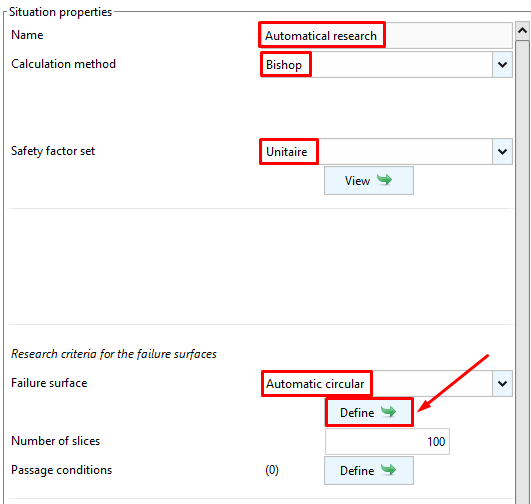
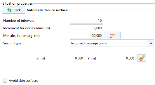
The range of failure surfaces to be examined is to be defined as follows:
We have defined everything necessary to start the calculation.
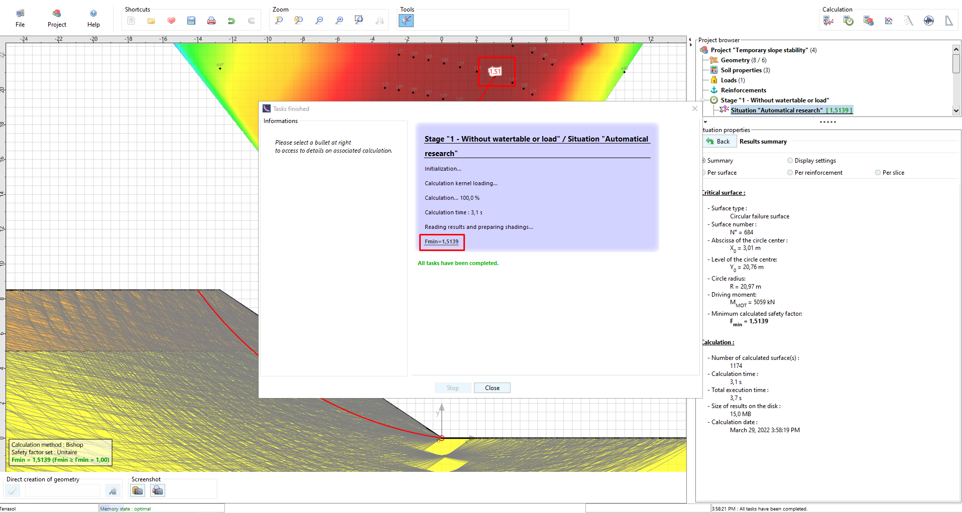
Select the situation and start the calculation using the first button in the calculation bar at the top of the window:
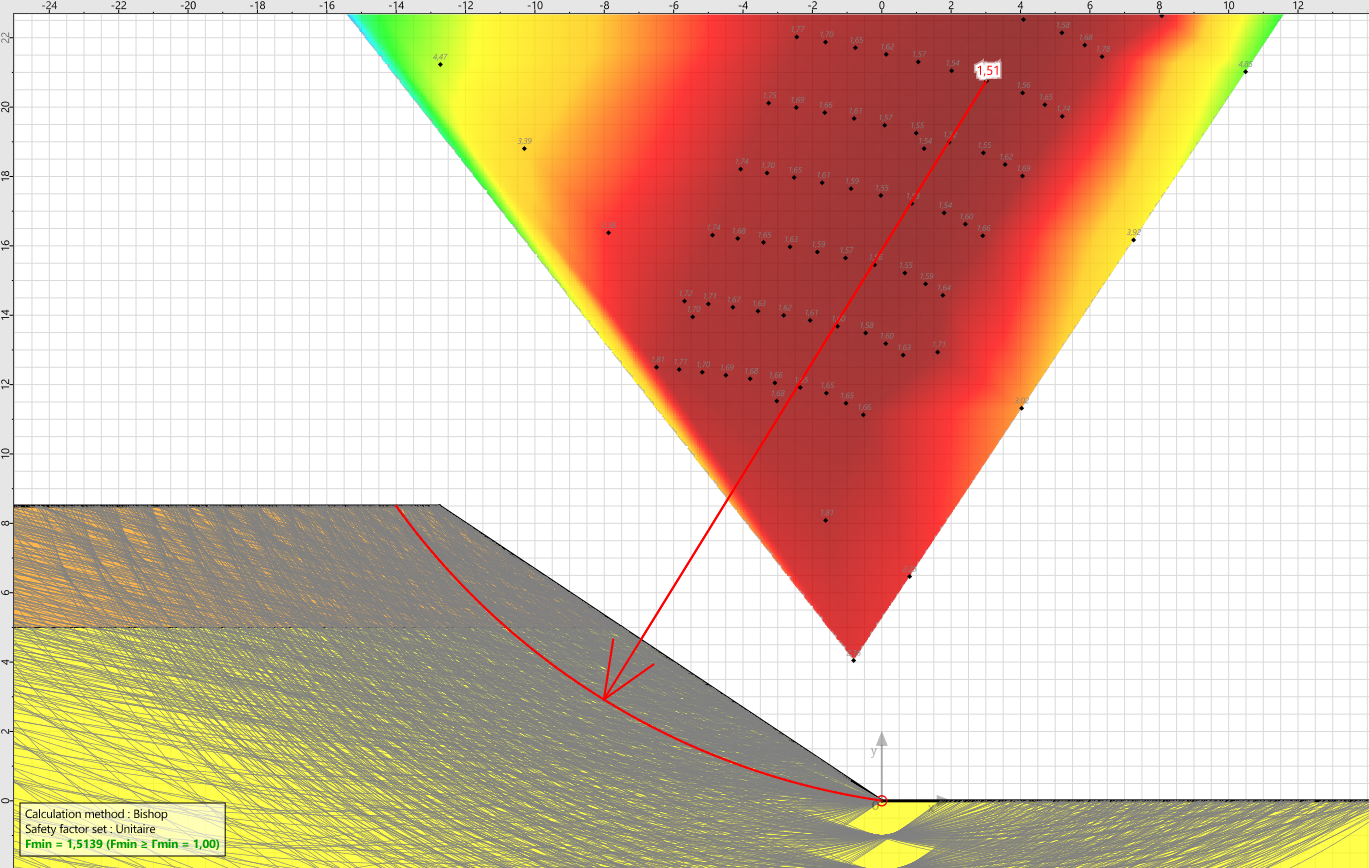
Once the calculation is completed, we obtain the safety coefficient Fmin = 1.51 and the associated mechanism:
Stage 2: Influence of a external load on the surface
We will then examine the influence of a surface loading.
To do this, we will add a new Phase by activating the external load:
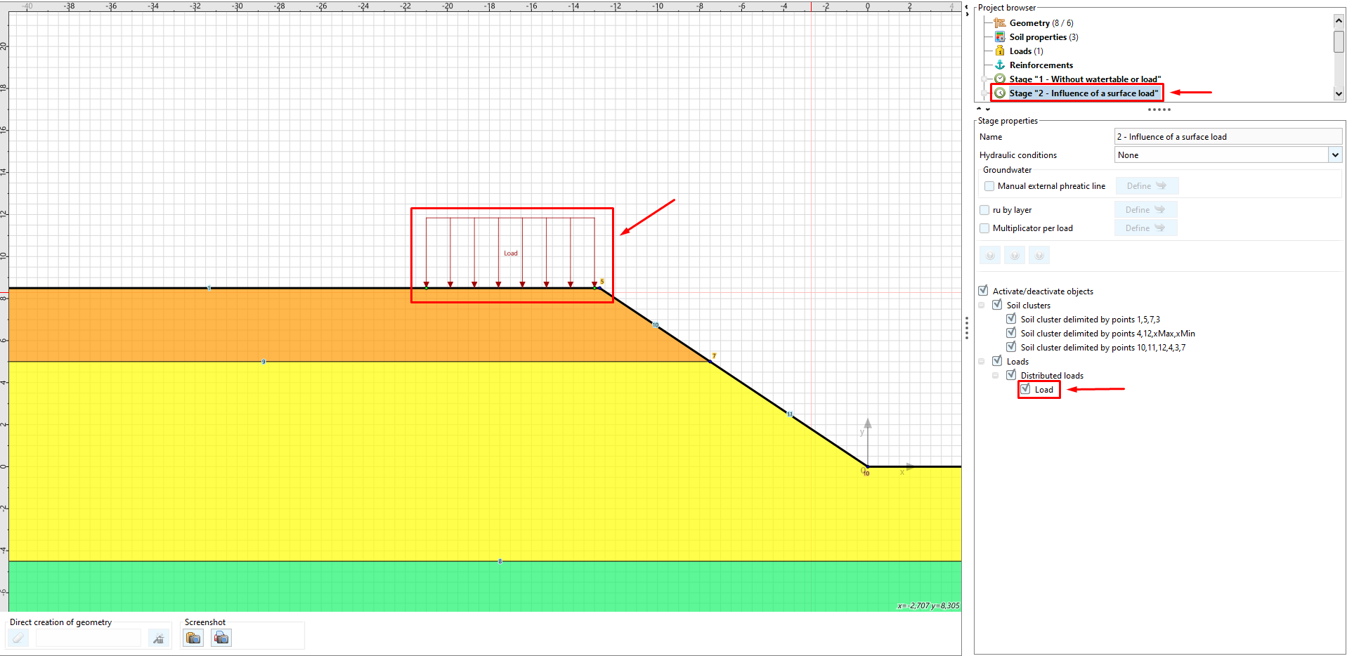
We then add a new situation by choosing this time a manual circular search:
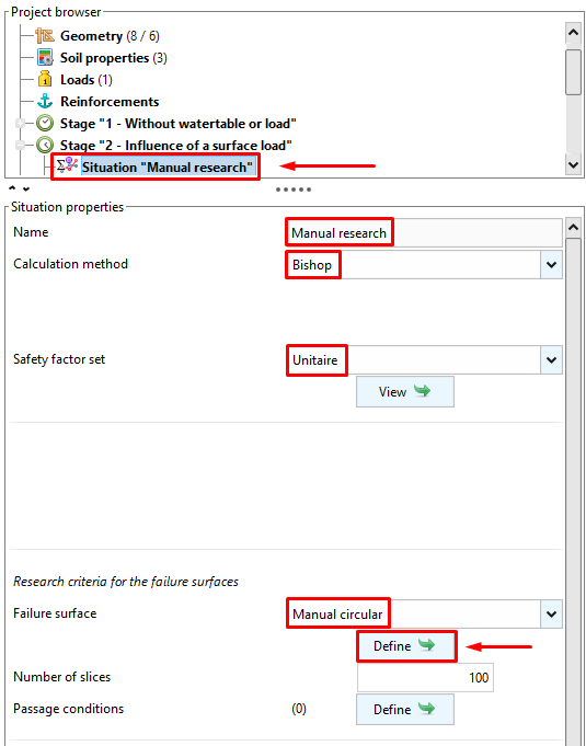
The parameters of the manual circular search are as follows:

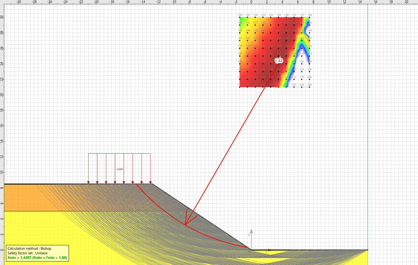
After calculation, we obtain a safety coefficient Fmin = 1.43.
Interpretation of the result: the safety coefficient is lower than in the previous phase because of the surface loading.
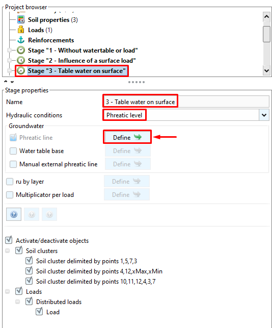
Stage 3: Influence of a horizontal water table
This phase aims at studying the stability of the structure in the presence of a horizontal water table at the level +8.50 m.
We will therefore create a new phase by defining phreatic conditions of the type Water Table:
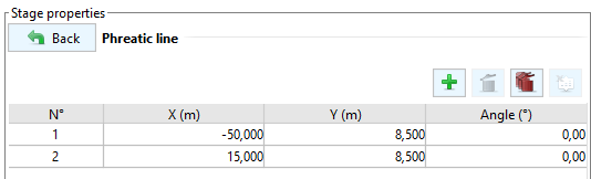
The coordinates of the points defining the water table are as follows:
We then add a new situation by choosing a manual circular search:
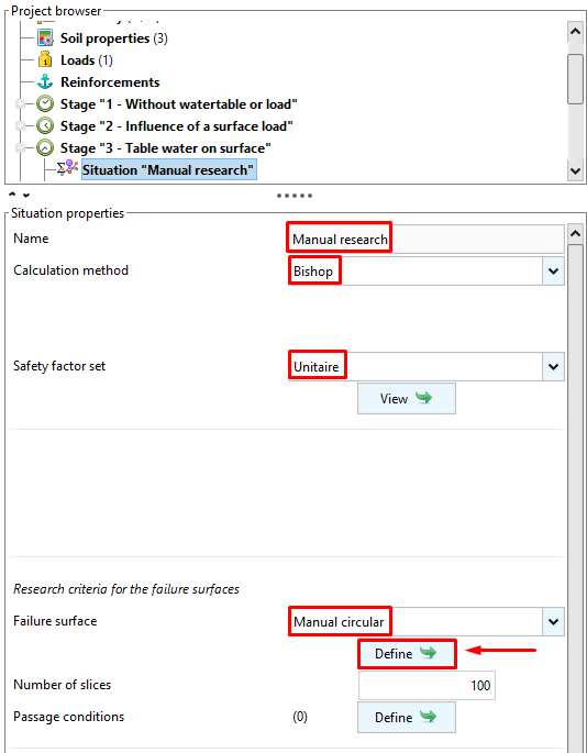
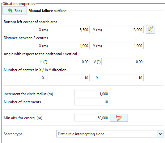
The parameters of the manual search are as follows:
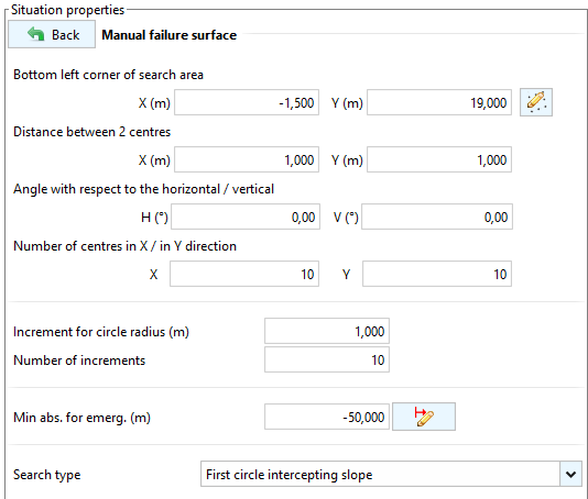
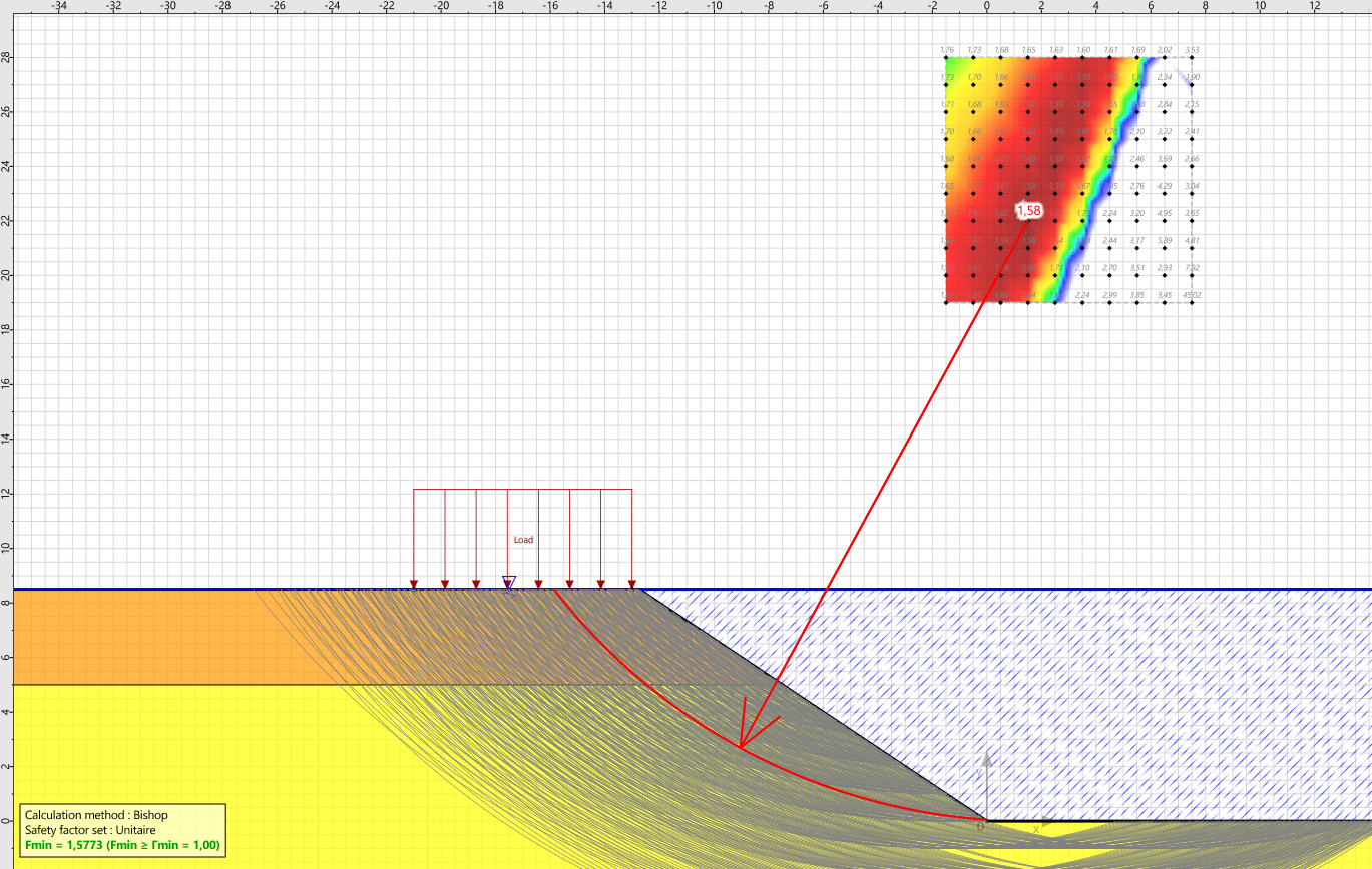
After calculation, we obtain a safety coefficient Fmin = 1.58.
Interpretation of the result: the obtained stability coefficient is higher than the previous ones due to the stabilizing character of the water weight on the right side of the model.
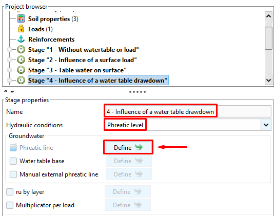
Stage 4: Influence of a water table drawdown
This phase aims at studying the stability of the structure in the presence of a lowering of the water table on the right side of the model.
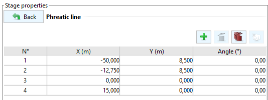
We will therefore create a new phase by defining phreatic conditions of the water table type following the profile of the natural ground:
The coordinates to be entered to define the water table are the following:
We then add a new situation by choosing a manual circular search:
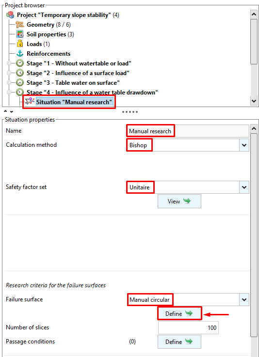
The parameters of the manual search are as follows:
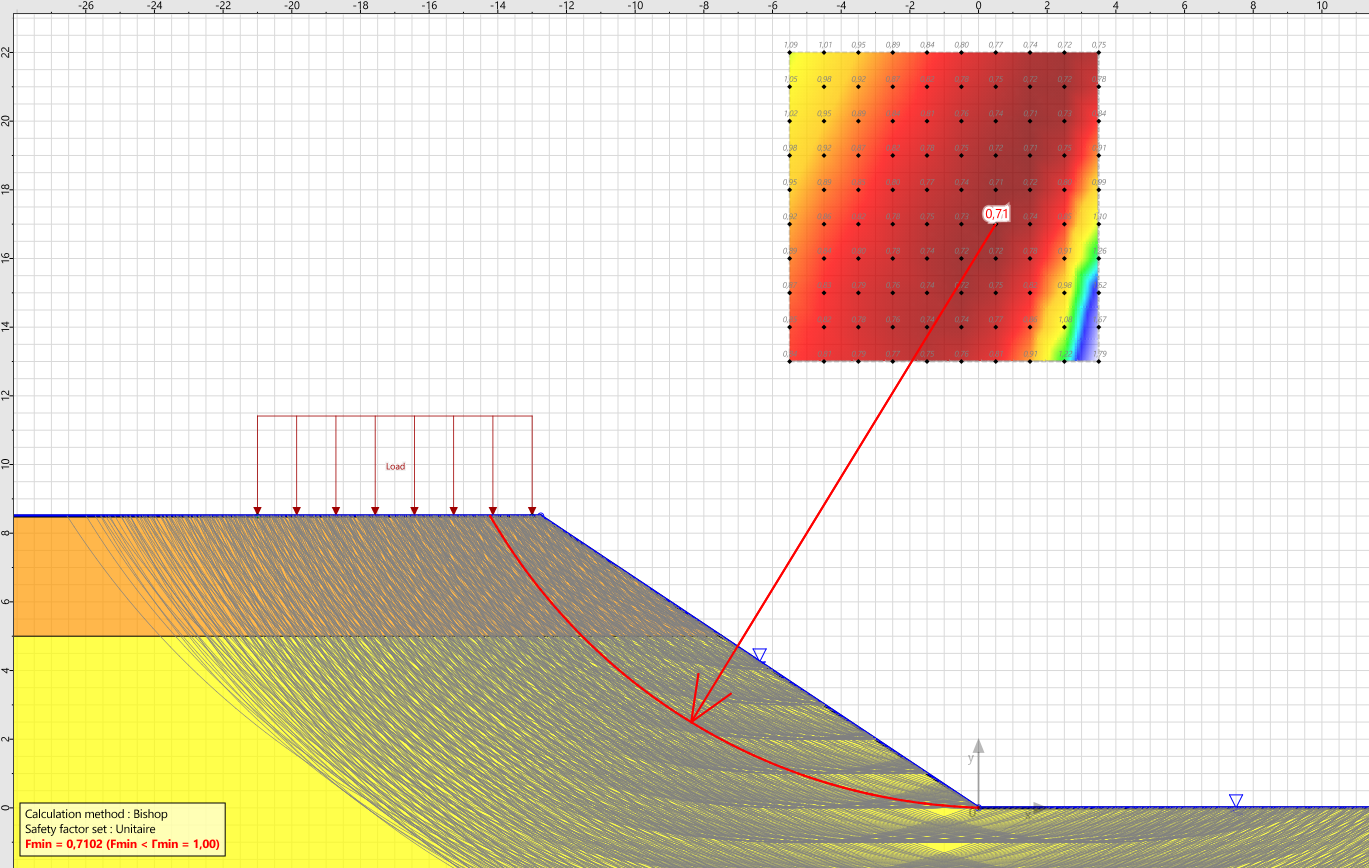
After calculation, we obtain a safety coefficient Fmin = 0.71.
Interpretation of the result: the stability coefficient is lower than that of the previous phases due to the removal of the favorable load of water to stability. It even remains lower than that obtained in phase 1 due to the fact that the effective stresses in the soil are lower due to the presence of water.
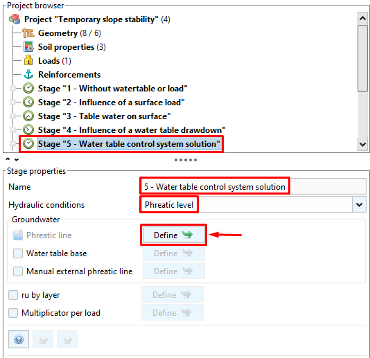
Stage 5: Interest of a water table control system
This phase aims to study the stability of the structure in the presence of a groundwater control system at the slope.
This system of control of the water table can be done by means of filtering points, drains, deep pumping...
We will therefore create a new phase by defining phreatic conditions of type Water table:
The coordinates to be entered to define the water table are the following:

We then add a new situation by choosing a manual circular search:
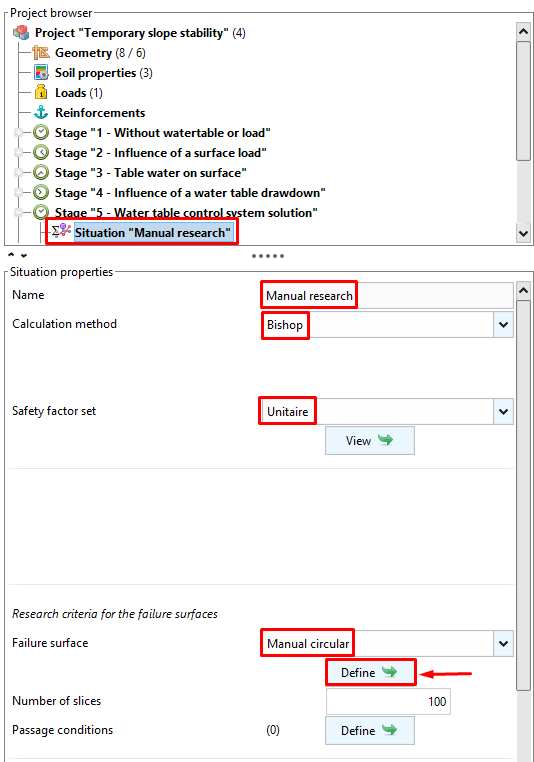
The parameters of the manual search are as follows:

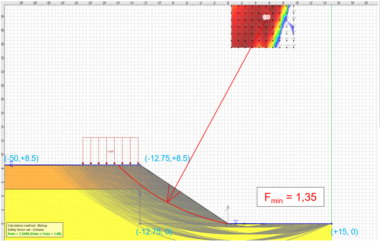
After calculation, we obtain a safety coefficient Fmin = 1.35.
Interpretation of the result: the stability coefficient is increased compared to the previous phase due to the fact that the effective stresses are higher under the sloping part because of the control of the hydraulic conditions. The water table control system thus shows its contribution towards the stability of the structure.
Stage 1 / Situation 2: calcul à la rupture (méthode cinématique)
After having analyzed the different stages planned for this structure, we propose to come back to phase 1 to study the stability using the kinematic method of calculation at failure.
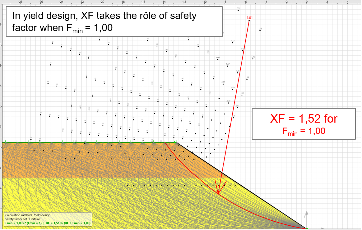
In the yield design, it is the XF coefficient that takes the role of safety factor when Fmin = 1.00.
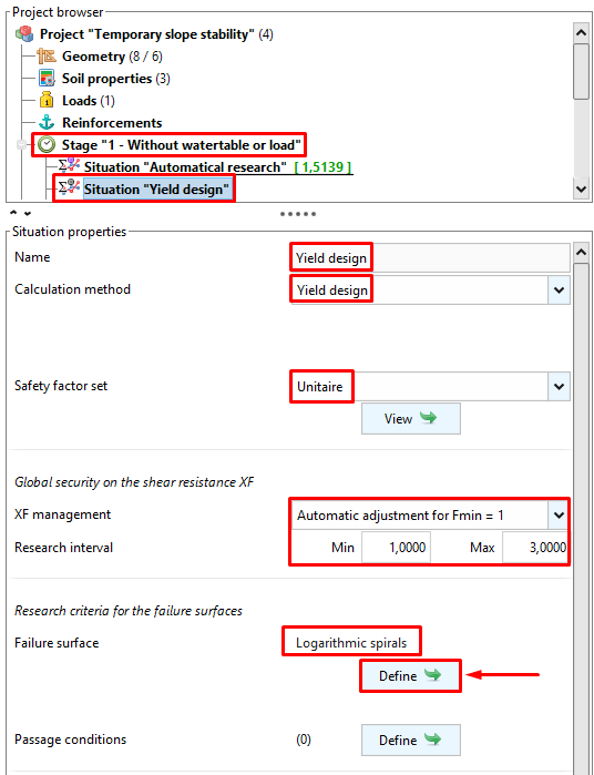
We will go back to phase 1 and add a new situation by choosing this time:
- Yield design
- Set of safety factors Unit
- Automatic adjustment of XF for Fmin = 1 over a search interval between 1.00 and 3.00
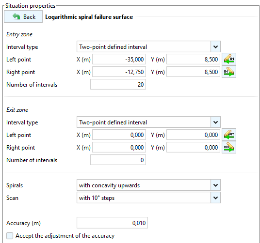
This method is implemented only for logarithmic spiral arc rupture mechanisms. The search parameters are summarized below:
After calculation, we obtain a safety coefficient of XF=1.52 for a stability coefficient of Fmin = 1.00.
Interpretation of the result: the level of security is of the same order and comparable to that obtained in Phase 1 / Situation 1 conducted using the slice method (Bishop).
Eurocode approach
How to use a set of partial coefficients?
In a semi-probabilistic approach (Eurocode 7 type for example), the shear properties of the soil are weighted at the source by a factor
Note that for a calculation leading to Fmin = 1.00, the safety margin is represented by the product
Physical interpretation of the result (applying a set of partial coefficients):
In practice, the model partial factor
- Γs3 for traditional slice methods (Bishop for example)
- XF for the yield design method
Stage 6 (identical to Phase 1): Without water table or loading
Situation 1: traditional method
We will create a new phase to study the same configuration as in phase 1 (without water table or loading) and then define a new situation with:
Bishop's method
Set of safety coefficients of type Eurocode - Fundamental - Standard
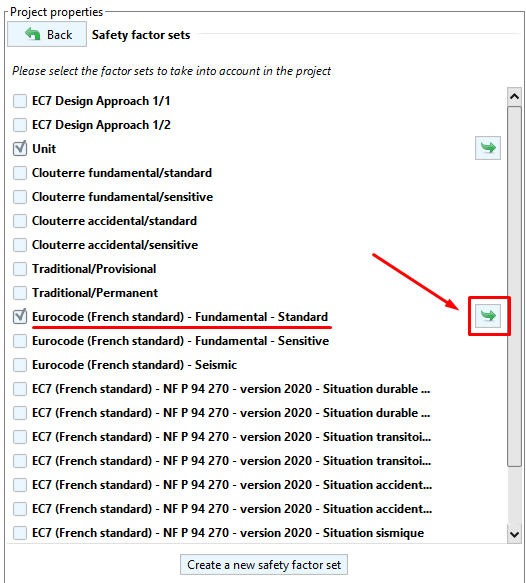
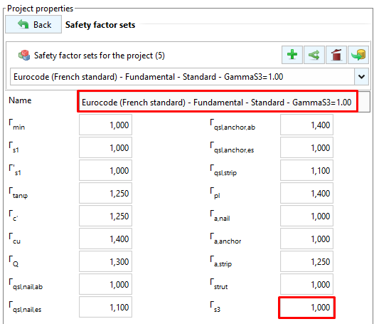
To use this set of safety factors, go back to the Project category and check it:
 img src="Talren_v6_Getting_started_guide.assets/image-20220324130433777.png" alt="image-20220324130433777" style="zoom:60%;" />
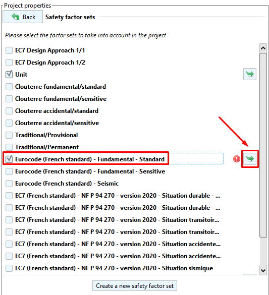
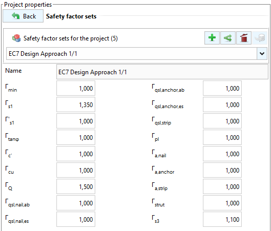
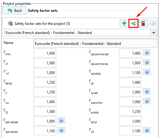
Since the Eurocode does not provide all the values of the coefficients, it is necessary to complete with unit values while knowing that these coefficients will not intervene in our calculation because there is no reinforcement:
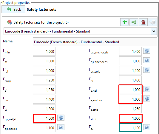
Very important: in slice method, the coefficient Γs3 plays the role of partial model factor. It is an additional security (overweighting of shear properties), here Γs3=1.1.
Situation definition:
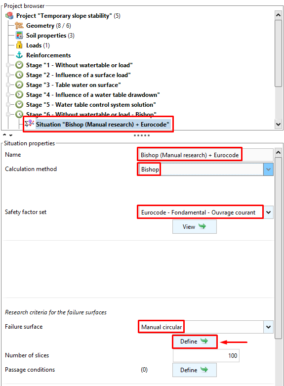
We will use the following failure surface search parameters:

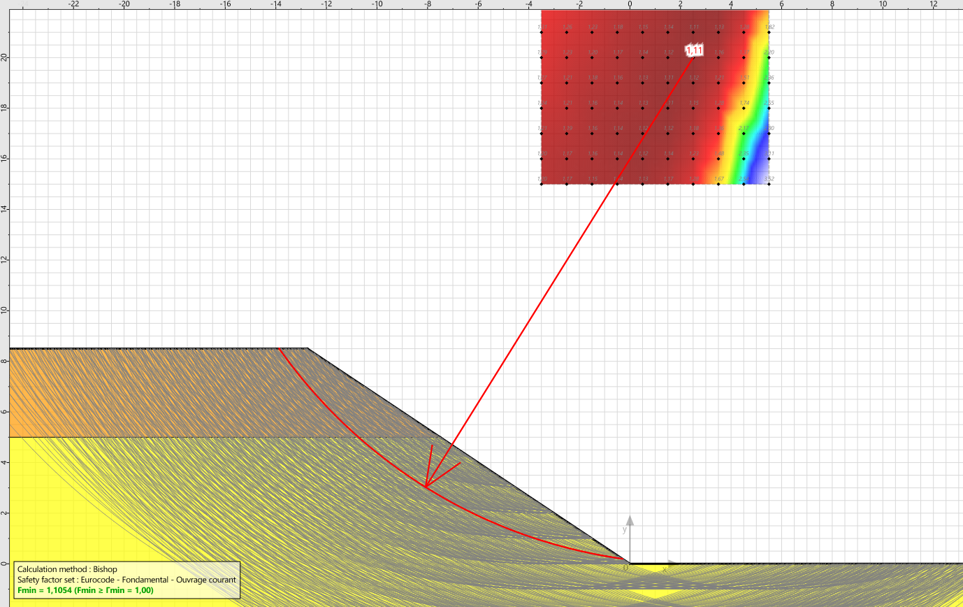
After calculation, we obtain
The overall security is calculated as follows:
x x = 1.25 x 1.10 x 1.1054 = 1.51 This value corresponds to the
value obtained with the traditional method.
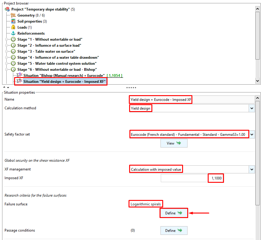
Situation 2: Yield design calculation (kinematic method) with imposed XF
We propose a step in the failure analysis to show how to apply it, first by imposing the value of XF and then by searching the value automatically.
Very important: in fracture calculation, the coefficient
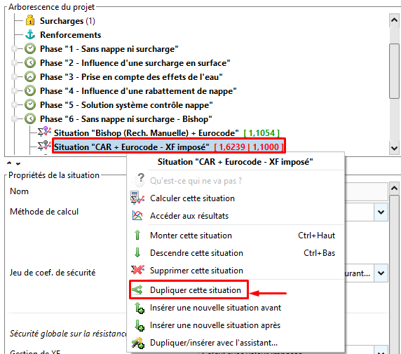
Procedure: in this new situation, we are about to validate that the required safety level is respected. To do this, we will create a new set of safety factors by duplicating the one used previously, while imposing
We return to the Project category and access the definition of the sets of safety coefficients:
Duplicate the set of safety coefficients and impose
We return to this new situation and choose this new set of safety coefficients, while imposing a value of
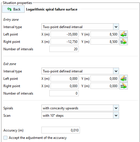
The parameters for generating the range of surfaces to be examined are as follows:
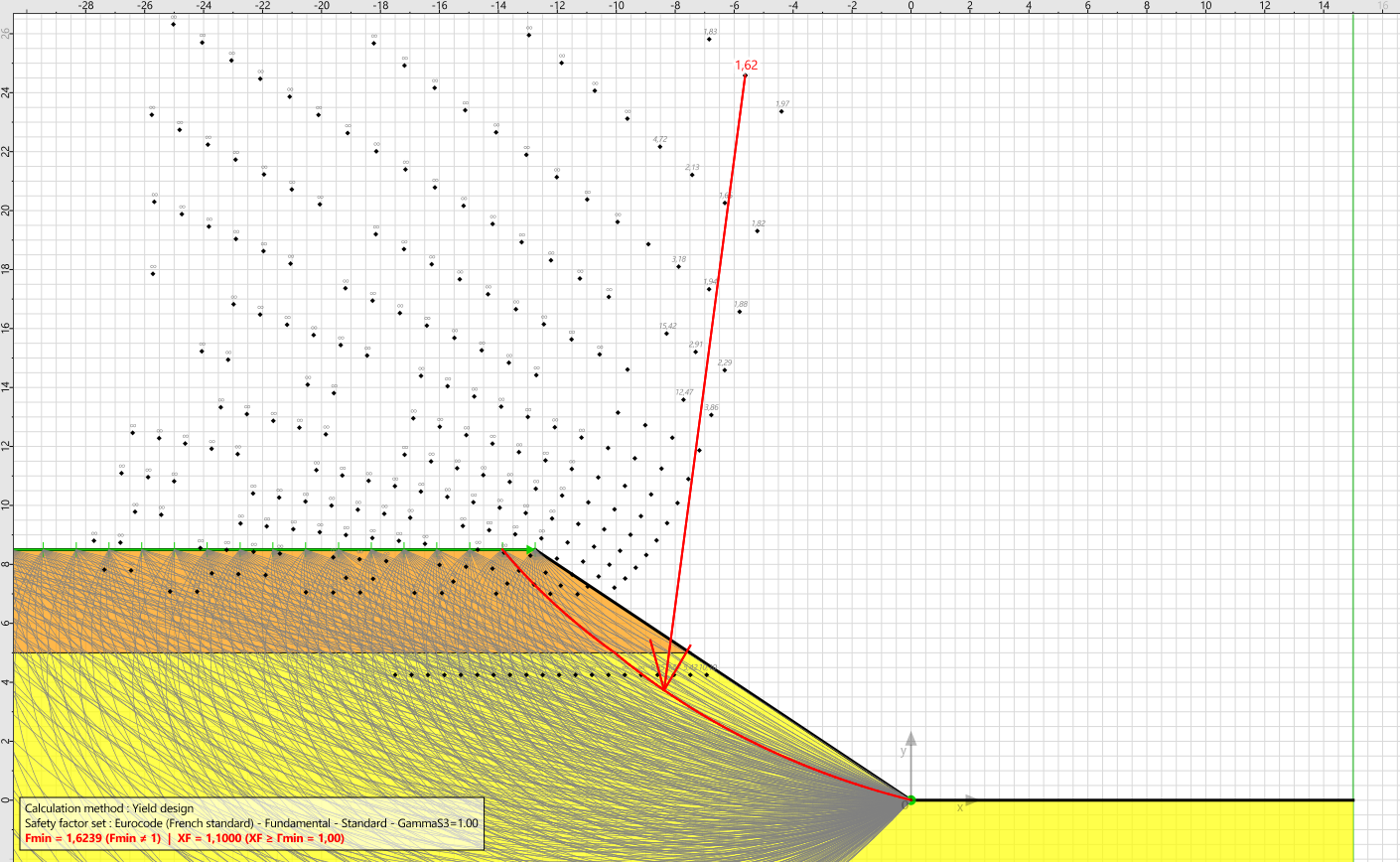
After calculation, we obtain
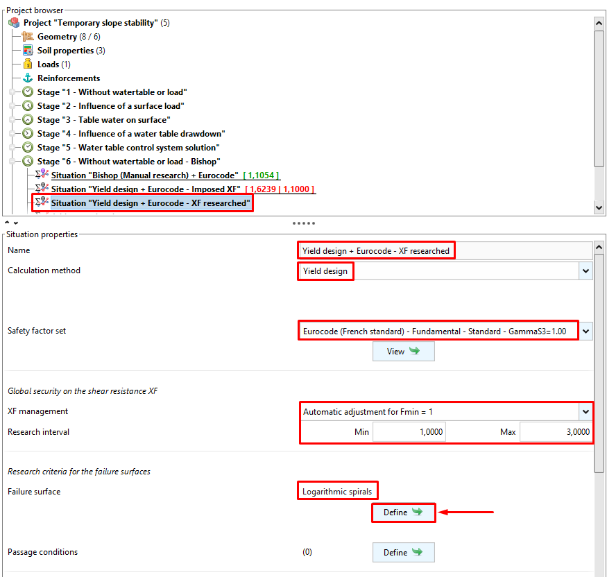
Situation 3: Yield design calculation (kinematic method) with automatic XF search
In this new situation, we propose to automatically find the safety level (XF) reached using the yield design method.
To do this, duplicate the previous situation:
We will still use the same set of partial coefficients as before (with Γs3=1.00) requesting an Automatic XF adjustment for Fmin = 1. Safety will be ensured if the obtained XF is greater than or equal to the targeted model partial factor.
The generation parameters of the surfaces to be examined remain unchanged.
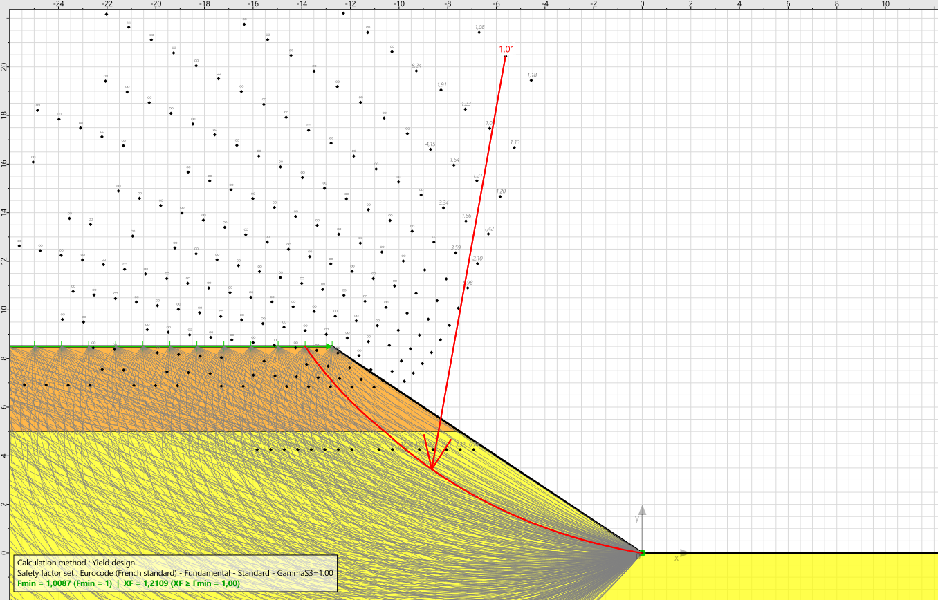
After calculation, we obtain XF=1.21 for
The global security is calculated as follows:
x x = 1.25 x 1.00 x 1.2109 = 1.51 This value corresponds to the
value obtained with the traditional method.
Want to go further?
This starting guide exposed the main features of the interface for a quick start.
The practical case (stability of a temporary slope) allowed to handle a simple project with Talren v6. We also discussed how to manage the level of safety in the traditional method, analyze the evolution of the safety factor throughout the proposed calculation phase. We have analyzed the stability using a set of partial coefficients according to Eurocode 7. Finally, we have compared the traditional method with the kinematic method of calculation at failure.
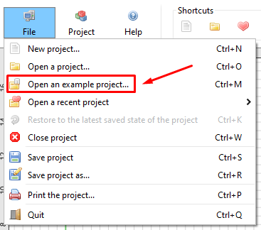
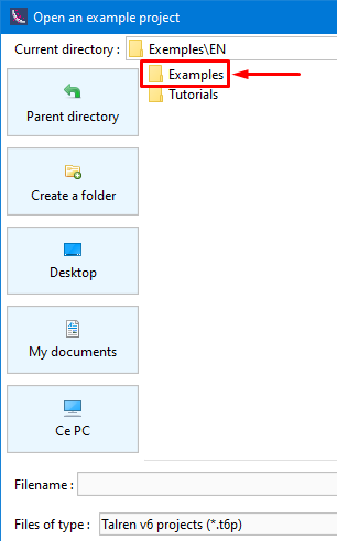
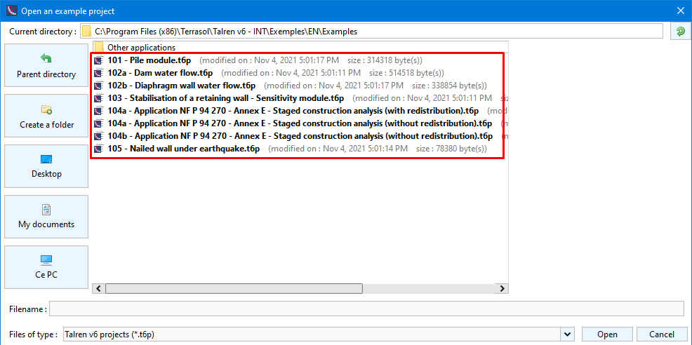
To go further, we invite you to consult the following examples provided with the interface:
They are accessible from the menu File / Open an example project.... / Examples subfolder:
Do not hesitate to contact us for any question at sales.terrasol@setec.com
![]()
Revision: March 2022