
Getting started with Slake
This document presents the general operation of the user interface to ensure a quick start for the user. The description of the calculation parameters and their choice is detailed in the software's scientific manual.
Getting started with SlakeGeneral operation of the interfaceHome screenWorkspaceCreating a project in SlakeSide panel for project and display managementProject definitionData set definitionParameters specific to CPT(u) data setsParameters specific to SPT data setsGraphical display of the data setCalculation results for a single data setResults as graphsGraphs available for CPT(u) data setsGraphs available for SPT data setsManaging the displayed graphsResults as tableResults synthesisCalculation results for multiple data setsResults as graphsComparison of multiple CPT(u) data setsComparison of multiple SPT data setsComparison of CPT(u) and SPT data setsComparison results as tableResults as isovalue mapsPractical considerationCopying and deleting a data setManaging the workspace and cards layoutHelp figures and tooltipsInformation messages and input controlGraphical display settingsInput table and data importManagement of the input tablesData import wizardKeyboard shortcuts
General operation of the interface
In Slake, the user works with different projects (saved as *.slkp files). A project includes a set of global parameters and may contain data sets for different soundings (CPT(u) and/or SPT tests). For each data set, an individual analysis can be carried out to determine the factor of safety at the depths of measurement. The results are presented in the form of graphs or tables.
In the case of a project containing several data sets, the comparison mode provides access to a comparative analysis in the form of graphs, tables, or plan representations of the results of the analysis for each sounding.
Home screen
The home screen offers various actions and information as shown below.
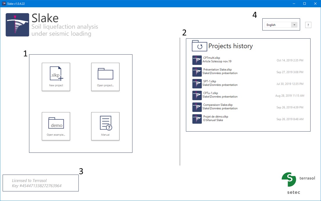
This group allows you to : * create a new Slake project
open an existing Slake project (project in *.slkp format)
open one of the example projects provided at the installation
- access the user manual
The project history area allows quick access to previously created and saved projects. They are listed in ante-chronological order with a reminder of the registration folder and of the last modification date.
License information is recalled here, including: the name of the company that owns the license used, the license key number and the expiration date, if any. By clicking on this area, the information is copied to the clipboard for easy transmission to the technical support department when assistance is requested.
The drop-down list allows you to choose the language of use of the interface: French or English.
Workspace
The workspace regrups 5 zones that are described in more detail below.
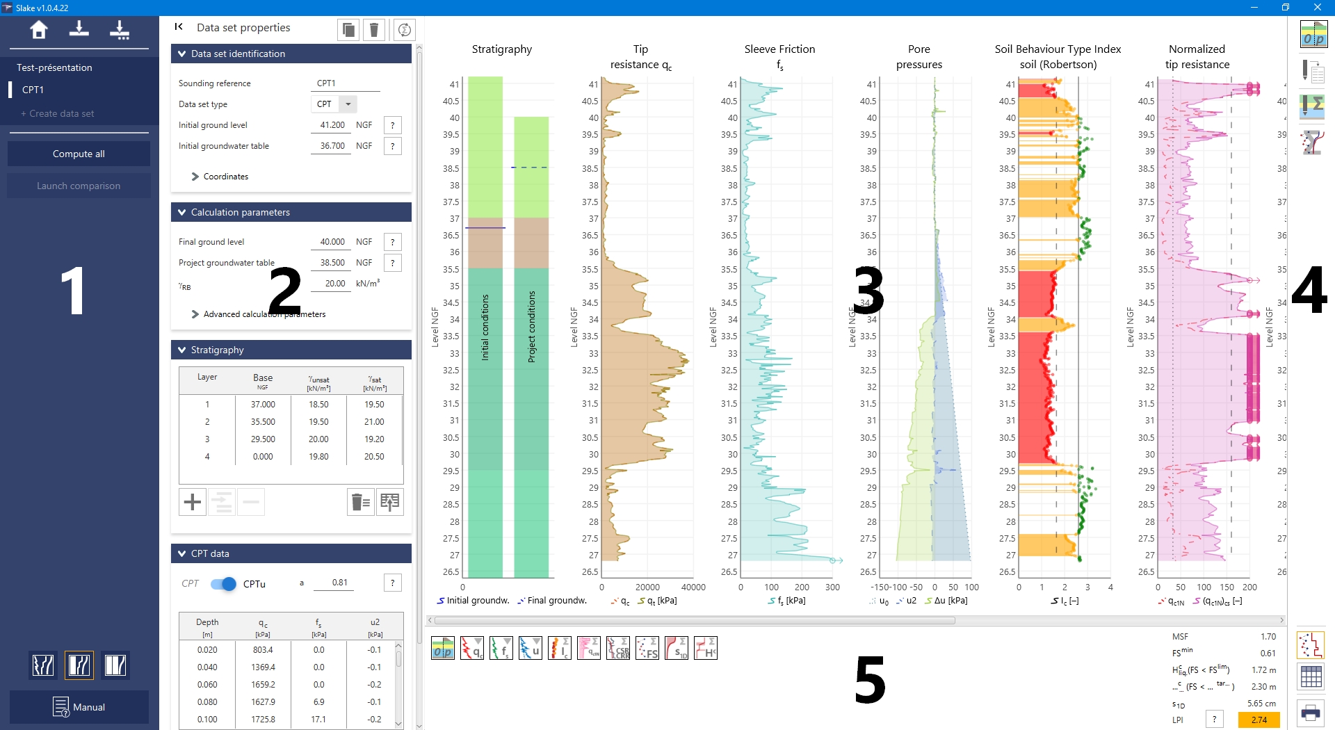
- The side panel for project and display management
- The input panel for calculation parameters (of projects and data sets)
- The results display area (in graphical or tabular form)
- The results display control panel
- The area for managing graphical displays and summarizing results.
Creating a project in Slake
Side panel for project and display management
Once a project has been created or opened, the user has access to various options and information via the side panel on the left of the interface.

From top to bottom, this panel gathers:
- The buttons for returning to the home screen (Ctrl+W), saving the project (Ctrl+S) and saving as... the project (Ctrl+Shift+S).
- The project tree area allowing access to the project definition screen, as well as to the various datas sets contained in the project. At the bottom of this area, the "+ Create a data set" button allows you to add a new data set to the project.
- The "Calculate all" button allows you to start calculating the results for all the data sets in the project. The "Start comparison" button allows you to access the comparison mode presented later in this manual.
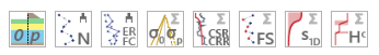
- The button group
 allows to switch between different display modes. The active mode is circled in orange.
 - The "Manual" button ensures easy access to the user manual and the software's technical manual.
Project definition
The project definition screen contains 4 input cards as shown below.

- Project identification: these text fields are used to indicate the project references as well as the elevation reference. This is used in the interface, in particular for the definition of levels and the f presentation of results.
- Calculation options: this card shows the choice of methods used in the project for the calculation of the factors of safety and the calculation of settlements. The parameters entered here by the user are used for the calculation related to each of the project's data sets.
- Seismic hypothesis: these parameters describe the seismic conditions to be taken into account in the calculations. The parameters entered here by the user are used for the calculation related to each of the project's data sets.
- Advanced parameters: this card allows you to access the definition of global parameters necessary to perform the calculation. In principle, the default values do not need to be modified but remain accessible to the user. The parameters entered here by the user are used for the calculation related to each of the project's data sets.
Once the project parameters have been defined, the user can create a new set of data using the "Create a data set" button.
Data set definition
The data set definition screen varies depending on the type of test considered: Slake allows cone penetration test (CPT or CPT(u) with piezocone) and standard penetration tests (SPT) to be taken into account. The 3 input cards presented below are common to both types of tests.

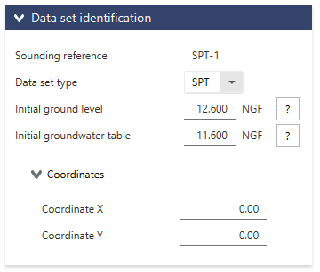
- Data Set Identification: This map allows you to fill in the sounding identification reference, the test type, as well as field and groundwater levels at the time of the sounding.
- Calculation parameters: this map describes the project conditions that will be taken into account in the calculation. Changing the advanced calculation parameters is not recommended but remains accessible by unfolding the corresponding area.
- Stratigraphic model: this map describes the stratigraphic model used in the calculations. The stratigraphic profiles under initial and project conditions are presented in the graphs area on the right-hand side of the screen.
Parameters specific to CPT(u) data sets
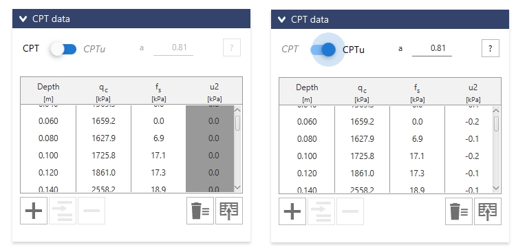
The "CPT data" card allows the static penetration test results to be entered (or imported) in a table. The user must specify wheter the test was conducted using a mechanical cone (CPT) or a piezocone (CPTu), in which case the u2 pore pressure values are needed. In the case of a CPTu data set, the user must enter the geometric correction parameter for overpressure "a" depending on the type of probe used. An indicative value is set by default.
Parameters specific to SPT data sets
Two input cards are specific to SPT soundings.
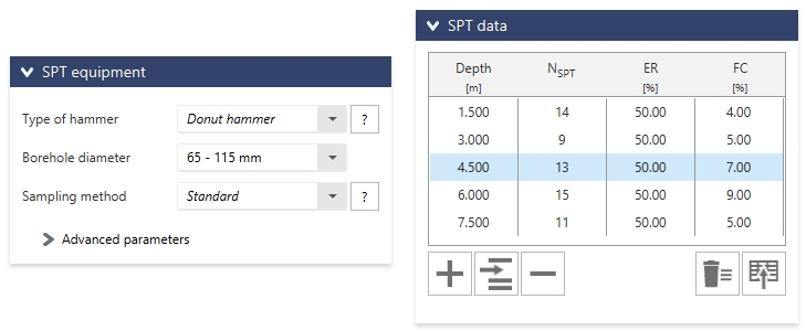
The "sounding diameter" and "sampling method" are necessary for the conduct of the analysis (they are used to calibrate corrective factors on the SPT blow count). The "type of hammer" is optional and used to estimate the the energy ratios ER if left empty in the SPT data table. The user defined ER values, if entered in the SPT data table, are systematically given priority to over the estimation method.
Graphical display of the data set
The input of a data set is automatically represented in graphical form. By default, the following data is shown:
In the case of a CPT data set:
- Stratigraphic and piezometric profiles under initial and project conditions
- The tip resistance profile
- The sleeve friction profile
- The pore pressure profile
In the case of an SPT data set:
- Stratigraphic piezometric profiles under initial and project conditions
- The SPT blow count
- The energy ratio and fines content
When all the data has been entered, the user accesses the "Calculate" button to activate the presentation of the analysis results.
Calculation results for a single data set
By default, the results are displayed in the form of graphs. It is possible to switch between the different display modes using the table  or graphs
  buttons located in the right side panel.
Results as graphs
Graphs available for CPT(u) data sets
The graphs available for CPT data sets are divided into 4 groups in the right side panel:
 Stratigraphic and piezometric profiles under initial and project conditions
 Display of the data set (input parameters)
 Data exploitation (complementary processing of the input data)
 The results of the liquefaction analysis itself
| Group | Pictogram | Name of the graph | Displayed by default before calculation | Displayed by default after calculation |
|---|---|---|---|---|
| | Stratigraphic and piezometric profiles | ✓ | ✓ |
|  | Tip resistance profile | ✓ | ✓ |
|  | Sleeve friction profile | ✓ | |
|  | Friction ratio profile (%) | ||
|  | Initial stresses and final stresses (project conditions) profiles | ||
|  | Soil Behaviour Type Index (Robertson) | ✓ | |
|  | Normalised tip resistance | ||
|  | CPT-based Soil Behaviour-Type Chart (Robertson) | ||
|  | Cyclic Stress Ratio and Cyclic Resistance ratio profiles | ||
|  | Factor of Safety profile | ✓ | |
|  | Post-liquefaction settlements | ✓ | |
|  | Cumulative thickness of liquefiable soils | ||
|  | CPT Clean Sand Base Curve for liquefaction for a reference magnitude |
Due to their format, the CPT-based Soil Behaviour-Type Chart (Robertson) and CPT Clean Sand Base Curve for liquefaction can only be displayed in solo mode by selecting the associated pictogram.
Graphs available for SPT data sets
- Stratigraphic and piezometric profiles under initial and project conditions
 Display of the data set (input parameters)
- Initial stresses and final stresses (project conditions) profiles
- The results of the liquefaction analysis itself
| Group | Pictogram | Name of the graph | Displayed by default before calculation | Displayed by default after calculation |
|---|---|---|---|---|
| | Stratigraphic and piezometric profiles | ✓ | ✓ |
 |  | SPT blow count | ✓ | ✓ |
|  | Energy ratio and fines content | ✓ | |
| | Initial stresses and final stresses (project conditions) profiles | ||
| | Cyclic Stress Ratio and Cyclic Resistance ratio profiles | ||
| | Factor of Safety profile | ✓ | |
| | Post-liquefaction settlements | ✓ | |
| | Cumulative thickness of liquefiable soils | ||
| | CPT Clean Sand Base Curve for liquefaction for a reference magnitude |
Due to its format, the CPT Clean Sand Base Curve for liquefaction is only displayed in solo mode.
Managing the displayed graphs
The area under the graphs area indicates the displayed graphs. Clicking on the pictogram of one of these graphs will center the display on it. The full title of each graph is displayed on hovering in the form of a tooltip.
 /
/ 
The right side panel gives control over the graphs displayed. The groups of graphs are unfolded at the left click to allow you to select the graphs to display. It is also possible to disable or activate all the graphs in a same group with a "click-wheel" or a right click to access a dedicated context menu.
Results as table
All input data, intermediate results and analysis results are available in a table format. The display of the results in table form is activated with the button  in the right side panel. The results table can be exported as a *.csv (or simply copied to the clipboard) file by clicking on the button
  for external data post-processing.
Results synthesis
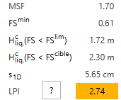
A summary of the results is available in the lower panel and includes:
- the reminder of the MSF value (Magnitude Scaling Factor)
- The minimum safety factor calculated at all test points of the sounding
- The cumulative liquefiable heights with respect to the limit factor of safety ()
- The cumulative liquefiable/sensitive heights with respect to the target factor of safety defined in the project parameters ()
- Estimation of post-liquefaction settlement
- The value of the liquefaction potential of the tested sounding, Liquefaction Potential Index (Iwaski et al. 1978)
Calculation results for multiple data sets
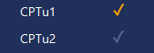
If two data sets are fully and correctly filled in, Slake offers to access a comparison mode from the "Launch comparison" button in the left side panel. By clicking on this button, all correctly defined data sets are calculated and selected for comparison.
A data set can be added or removed from the comparison by clicking on the ✓ button adjacent to it in the left side panel.
By default, the comparison results are displayed in the form of graphs (superposition of the result curves). It is possible to switch between the different display modes using the table , graphs or isovalue map  buttons in the right side panel. To access the plane representations it is necessary to use a minimum of 3 data sets, including their (X, Y) coordinates which are par of the "Data set identification" card:
Results as graphs
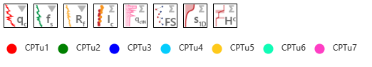
In graph mode, the comparison mode overlays the graphical results plotted for each of the selected data sets. The lower side panel contains the legend to identify each set.
Comparison of multiple CPT(u) data sets
The following is a list of graphs available when the project contains only CPT(u) data sets.
| Group | Pictogram | Name of the graph | Displayed by default |
|---|---|---|---|
| | Tip resistance profile | ✓ |
| | Sleeve friction profile | |
| | Friction ratio profile (%) | |
| | Soil Behaviour Type Index (Robertson) | ✓ |
| | Normalised tip resistance | |
| | CPT-based Soil Behaviour-Type Chart (Robertson) | |
| | Factor of Safety profile | ✓ |
| | Post-liquefaction settlements | ✓ |
| | Cumulative thickness of liquefiable soils | |
| | CPT Clean Sand Base Curve for liquefaction for a reference magnitude |
Comparison of multiple SPT data sets
The following is a list of graphs available when the project contains only SPT data sets.
| Group | Pictogram | Name of the graph | Displayed by default |
|---|---|---|---|
| | SPT blow count | ✓ |
| | Energy ratio and fines content | |
| | Factor of Safety profile | ✓ |
| | Post-liquefaction settlements | ✓ |
| | Cumulative thickness of liquefiable soils | |
| | CPT Clean Sand Base Curve for liquefaction for a reference magnitude |
Comparison of CPT(u) and SPT data sets
The following is a list of graphs available when the project contains both CPT(u) and SPT data sets.
| Group | Pictogramm | Name of the graph | Diplayed by default |
|---|---|---|---|
| | Factors of Safety | ✓ |
| | Post-liquefaction settlements | ✓ |
| | Cumulative thickness of liquefiable soils | ✓ |
| | CPT Clean Sand Base Curve for liquefaction for a reference magnitude |
Comparison results as table
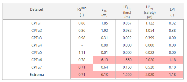
The tabular display shows the summary results for each data set and highlights the extreme values and associated data sets.
Results as isovalue maps
From 3 selected data sets, the comparison mode allows a representation in the form of an analysis isovalue map. The data sets are positioned in plan according to the X and Y coordinates in the "Data set identification" card. Iso-values are determined from the interpolation of the results for each data set.
The following results can be visualized:
- The minimum safety factor calculated for each data set
- The cumulative liquefiable heights with respect to the limit factor of safety ()
- The cumulative liquefiable/sensitive heights with respect to the target factor of safety defined in the project parameters (
- Estimation of post-liquefaction settlement
- The value of the liquefaction potential LPI (Iwaski et al. 1978)
Practical consideration
Copying and deleting a data set
Within a project, data sets can easily be duplicated or deleted. Two methods exist:
- in the side panel, right-click on the data set name to access a contextual menu for duplication or deletion
- in the data set definition panel, two buttons allow you to duplicate the data set
 or remove it
Managing the workspace and cards layout
The group of buttons in the side panel allows you to switch between different interface layouts to optimize the display according to your hardware and the task performed (input or evaluation).
 gives priority to the results by folding back the panel containing the input cards.
  forces the display of input cards on a single column to allow a good balance between access to calculation data and results. This display mode is enabled by default when the calculating a data set.
  gives priority to the input panel that will take up the space necessary to display all the cards.
It is also possible to fold up/unfold the input cards by clicking on their header to manually optimize the display.
Help figures and tooltips
Some parameters have an associated help figure to help the user in defining them. The help figures are accessible with the  buttons. The help figure is automatically closed with a single click anywhere on the screen.
All parameters whose title is not explicit on the interface are also explained using a text tooltip that appears on hovering. This tooltip system is also used for action buttons or for graphs selection.
Information messages and input control
Throughout the editing of a project, the data entered by the user is checked and warnings are displayed to the user:
- when changing an advanced parameter
- when entering an incorrect value
- when data are missing.
If the entry does not allow the calculation to be completed, the warning will be displayed in red, while the warnings displayed in orange inform the user of an possibly inconsistent value or one that requires the calculation to be restarted.
The side panel uses this color code to inform the user about the status of the data set. An orange dot  informs the user that the data set needs to be recalculated, while a red dot
  specifies that the input data does not allow the calculation to start.
Graphical display settings
For all results displayed in graph format, the interval (min, max) of the displayed entities on the x-axis can be changed manually. Right-click on the graph to access the "horizontal axis configuration" option. It is then necessary to configure the minimum and/or maximum bounds of the abscissa to be projected.
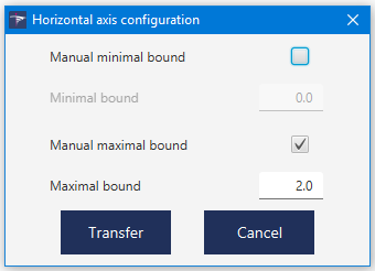
Note that by unticking the manual input options, Slake will project the abscissa with the intervals set by default for each graphic. This option is also valid for the planar representation of the results, where it becomes possible to define an interval for both the x-axis, y-axis, and color scale of the projected calculation result.
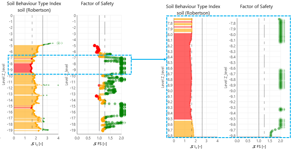
It is also possible to zoom in on all the graphics (y-axis) directly with the mouse wheel.
Input table and data import
Management of the input tables
The input tables for stratigraphic models and individual data set exploitation are used with different action buttons located below.
 adds a line at the end of the table
 inserts a line before the selected line
 deletes the selected line
 deletes all lines in the table
 brings up the import wizard window.
Data import wizard
The import wizard allows you to import data from the clipboard. This data may have been copied from Excel or from a text file that uses the "tabulation" character as a column separator.
When the wizard is launched, the contents of the clipboard are read and the columns are identified
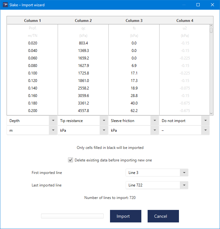
For each of the identified columns, the user matches it to a column of the table, and specifies the unit of the data to be imported. This last operation ensures the conversion into the units used by the software. The user can also specify the interval of lines to be imported, in particular to avoid importing any header lines from the clipboard.
Keyboard shortcuts
| Combination | Action |
|---|---|
| Ctrl+N | New project |
| Ctrl+O | Open project |
| Ctrl+S | Save project |
| Ctrl+P | |
| Ctrl+W | Back to home screen |
| Alt+F4 | Close Slake |
![]()